Shape Recognition with ShapeFinder

Table of Contents

• Introduction
• Prerequisites
• Train a pattern
• Search for patterns
• Parameters
• Examples

C++	.NET	Python
Cvb::ShapeFinder2	Stemmer.Cvb.ShapeFinder	cvb.shapefinder2

Introduction

ShapeFinder is a search tool to find previously trained objects in newly acquired images. The algorithm is designed following the principles of the Generalized Hough Transform (GHT).

ShapeFinder returns the object location with subpixel accuracy as well as the rotation angle and the scaling of the object(s) found. One particular feature of the software is its tolerance to changes in the object that may appear in production lines such as:

• partially covered object areas,
• noise or
• reflections.

The user has the choice between an extremely fast or a slightly slower but more accurate and more reliable recognition.

Prerequisites

ShapeFinder generally operates on images provided by the Common Vision Blox Image Manager. The input images, however, must meet certain criteria for ShapeFinder to work on them:

1. The pixel format needs to be 8 bit unsigned.
2. ShapeFinder works on one single image plane, i.e. it expects a monochrome image.

Train a pattern

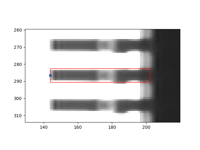
The CVB APIs provide functions to train a dedicated pattern with ShapeFinder. To do this, a point must be given in the image that specifies the position of the pattern and an axis-aligned rectangular region that contains the pattern. The region is always specified relative to the point, i.e. in the form of the values left, top, right, bottom.

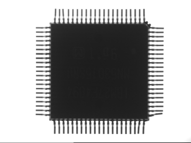
The following code gives an example of how to train the pin of a computer chip. The aim of the example is to find all pins and determine their rotational positions. For training, we select a random pin from the left side of the chip.

The example image.

C++C#Python

C++

#include <iostream>
#include <cvb/shapefinder2/classifier_factory.hpp>
#include <cvb/shapefinder2/classifier.hpp>
 
int main()
{
    auto testimage = Cvb::Image::Load(Cvb::InstallPath() + CVB_LIT("Tutorial/ShapeFinder/Images/SF2/Chip/Chip3.bmp"));
 
    int x0 = 144;          // the pattern position
    int y0 = 286;
    int left = 0;          // the pattern region relative to the position
    int top = -4;
    int right = 58;
    int bottom = 4;
 
    // Create a shapefinder classifier from image, point and region
    auto clf_fac = Cvb::ShapeFinder2::ClassifierFactory();
    auto clf = clf_fac.Learn(testimage->Plane(0), Cvb::Point2D<int>(x0, y0), Cvb::Rect<int>(left, top, right, bottom));
    .
    .
    .

C#

using Stemmer.Cvb;
using Stemmer.Cvb.ShapeFinder2;
 
var testimage = Image.FromFile(Environment.ExpandEnvironmentVariables(@"%CVB%/Tutorial/ShapeFinder/Images/SF2/Chip/Chip3.bmp"));
 
int x0 = 144;          // the pattern position
int y0 = 286;
int left = 0;          // the pattern region relative to the position
int top = -4;
int right = 58;
int bottom = 4;
 
// Create a shapefinder classifier from image, point and region
var clf_fac = new ClassifierFactory();
var clf = clf_fac.Learn(testimage.Planes[0], new Point2D(x0, y0), new Rect(left, top, right, bottom));
.
.
.

Python

import os
import math
import cvb.shapefinder2
import matplotlib.pyplot as plt
from matplotlib.patches import Rectangle
 
if __name__ == "__main__":
    testimage = cvb.Image.load(os.path.join(cvb.install_path(), "Tutorial/ShapeFinder/Images/SF2/Chip/Chip3.bmp"))
 
    x0, y0 = 144, 286                           # the pattern position
    left, top, right, bottom = 0, -4, 58, 4     # the pattern region relative to the position
 
    # Create a shapefinder classifier from image, point and region
    sfcf = cvb.shapefinder2.ClassifierFactory()
    clf = sfcf.learn(testimage.planes[0], cvb.Point2D(x0, y0), cvb.Rect(left, top, right, bottom))
 
    # Display the trained region
    fig, ax = plt.subplots()
    ax.imshow(cvb.as_array(testimage), 'grey')
    rc = Rectangle((x0, y0 - bottom), right, abs(top) + abs(bottom), edgecolor='red', fill=False)
    ax.scatter(x0, y0)
    ax.add_patch(rc)
    plt.show()
    .
    .
    .

The above python code will produce the following image

Detail of the test image. The blue dot indicates the pattern position, the red rectangle the region.

Using the default settings, the classifier is created with complete rotational invariance and no scale invariance. This can be controlled by setting corresponding minimum and maximum values of the ClassifierFactory object. In this case, the classifier should find all pins, as they vary in their rotational position but not in their scaling.

Search for patterns

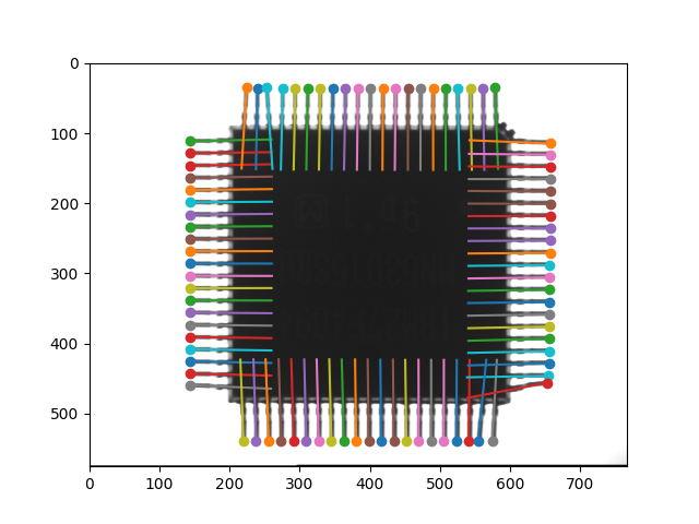
We examine the image by searching for all pins in the entire image area and determining their respective position and rotation.

C++C#Python

C++

    .
    .
    .
    auto search_res = clf->SearchAll(testimage->Plane(0), 
                                     testimage->Bounds(), 
                                     Cvb::ShapeFinder2::PrecisionMode::CorrelationFine, 
                                     0.55, 
                                     20, 
                                     5);
                                     
    for (int i = 0; i < search_res.size(); i++)
    {
        std::wcout << i << ": " << search_res[i].X() << "  " << search_res[i].Y() << "  " << search_res[i].Rotation().Deg() << "\n";
    }
}

C#

.
.
.
var search_res = clf.SearchAll(testimage.Planes[0], testimage.Bounds, PrecisionMode.CorrelationFine, 0.55, 20, 5);
for (int i = 0; i < search_res.Length; i++)
{
    Console.WriteLine("{0}: {1}, {2}, {3}", i, search_res[i].X, search_res[i].Y, search_res[i].Rotation.Deg);
}

Python

.
.
.
search_res = clf.search_all(testimage.planes[0], testimage.bounds,
                            precision=cvb.shapefinder2.PrecisionMode.CorrelationFine,
                            relative_threshold=0.55,
                            minimum_threshold=20,
                            coarse_locality=5)
 
# Display the results
plt.imshow(cvb.as_array(testimage), 'grey')
for res in search_res:
    startx = res.x
    starty = res.y
    alpha = res.rotation.rad
    endx = startx + 2*right*math.cos(alpha)
    endy = starty + 2*right*math.sin(alpha)
    plt.scatter(startx, starty)
    plt.plot([startx,endx],[starty,endy])
plt.show()

The above python code will produce the following image

The found pins with their orientations.

Parameters

Shapefinder operates on a certain pyramid layer of the original image, which is determined during the training process. The depth of the pyramid from which the training process selects the layer can be defined by the parameter MaxCoarseLayer. The layer actually selected can be retrieved after training under CoarseLayer.

Depending on which value is used for the Precision parameter in the search process, the results found on this coarse scale layer are processed further or not. The precision mode parameter influences the search process as follows:

1. PrecisionMode.NoCorrelation is the fastest search mode available. It ends when the search has been completed on the coarse layer in accordance with GHT. Since the positions of the coarse layer are converted to positions in the original image, there will inevitably be quantization deviations depending on the reduction of the resolution in the coarse layer.
2. In search mode PrecisionMode.CorrelationCoarse, the positions of all GHT results on the coarse layer are improved within the coarse layer grid by a correlation with the corresponding coarsened trained pattern. Although there are now results in the subpixel range, they still refer to the grid of the coarse layer and the corresponding statements regarding the conversion to the original resolution apply as above.
3. Finally, in mode PrecisionMode.CorrelationFine, the correlation between GHT results and the training pattern is actually calculated in the resolution of the original image. Subpixel accuracy and angular resolution are maximized here, at the price of a higher processing time.

The features which Shapefinder uses for pattern recognition are gradient magnitudes and directions. Accordingly, the minimum_threshold parameter in the search function refers to a minimum value for the gradient magnitude in order to be counted as a feature. The relative_threshold relates to the consideration of further search results relative to the best result, while the coarse_locality value describes a required minimum distance between two results.

Examples

Example	Description
QTShapeFinder2 (QML C++ version)	Detect screws (QML C++ version)
Python example	Detect screws (Python version)