
Common Vision Blox Foundation Package Tool
 C-Style |  C++ |  .Net API (C#, VB, F#) |  Python |
| CVCEdge.dll | Cvb::Foundation::Edge | Stemmer.Cvb.Foundation.Edge | cvb.foundation |
Image processing tool for Edge detection
The Edge Tool provides functions to detect edges within an image as well as functions to generate projections in any direction.
Three function groups are currently described in Edge:
All function groups primarily serve to perform edge-oriented image processing tasks.
The Edge Tool is only working on single planes of images (8 or more bit).
The search direction is determined by the position and orientation of the scan window. Subsampling is possible using the density parameter. In connection with the use of scan windows and sampling density, an understanding of the terms area and density as they are used in CVB is necessary.
Please refer to the chapters Area of interest AOI and Coordinate System and Areas, for a description supplementary to the present documentation.
Features
Explanation of projection and edge detection
Edge provides you all functions you might need to develop your own algorithm, such as direct access to the projection data, projection filtering and thresholding as well as functions to detect zerocrossings. They are described in the API. Optimal using these function needs knowledge of the edge parameter below :
In image processing, a projection is understood to be the summing of columns or rows within an image. The row or column totals are written into a buffer, which is then analyzed. Summing smoothes out unsharp edges, consequently enabling them to be analyzed.
The following example shows the projection of the columns for the gray values of a hypothetical AOI (area of interest). The AOI has a width of 10 pixels and a height of 3 pixels.
| 69 | 75 | 78 | 85 | 98 | 120 | 128 | 135 | 133 | 135 |
| 66 | 69 | 76 | 81 | 88 | 102 | 118 | 129 | 134 | 136 |
| 68 | 74 | 81 | 87 | 101 | 119 | 128 | 136 | 134 | 135 |
Viewed from left to right, the AOI represents a graduation from black to white. The middle row appears to be shifted slightly to the right, which could be attributable to the framegrabber used. This effect is referred to as jitter, and results from the imprecision of the PLL (phase lock loop). Independently for each row, this jitter causes a shift at the beginning of the row. As one can easily imagine, edge detection using just one row yields an imprecise result. If, on the other hand, the sum of the columns, that is to say the projection, is used for detection, the displaced middle row is averaged out.
| 203 | 218 | 235 | 253 | 287 | 341 | 374 | 400 | 401 | 406 |
The column totals divided by the number of rows gives us the normalized projection, the values of which are again on a scale of 0 to the maximum gray value (usually 255):
| 68 | 73 | 78 | 84 | 96 | 114 | 125 | 133 | 133 | 135 |
The following illustration shows a typical normalized projection; the projection data was written in each row of the AOI:
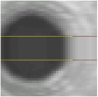
The functions for edge detection within the Edge Tool use the normalized projection. It may however also be useful to use non-normalized projection, for example for blob detection. A "blob" is an enclosed area whose pixels have approximately the same gray value (e.g. a white dot on a black background). To determine the position of the blob in a binary image, clearly one would then want to calculate the projections in the x and y directions. The position of the enclosing rectangle is obtained by searching in the horizontal and vertical buffer for the first and last values unequal to zero.
It is often possible to increase processing speed by subsampling the respective pixels. Given an area size of 512*512 pixels, the same number of additions are required to calculate a single projection. To calculate both projections, therefore, requires 524288 additions. If, however, only every second pixel in every second row is used to calculate the projection, the number of additions required falls to 256*256*2=131072, which significantly speeds up execution of the operation. The precision is of course lower, depending on the subsampling density.
Within the Edge Tool, this subsampling can be set using the Density parameter of the Edge detection functions.
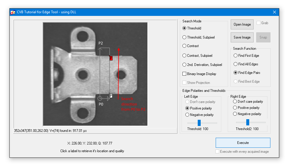
The direction of the projections is predetermined by the definition of the CVB area. An area is defined in CVB by the three points P0, P1 and P2.
The points generally describe a parallelogram of any orientation which is usually reduced to a - sometimes rotated - rectangle. The columns are summed in the direction P0-P1:
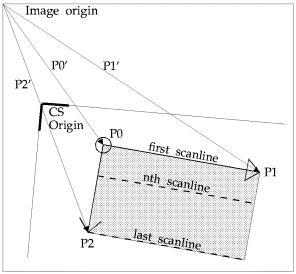
The Search Direction is defined from P0 to P2.
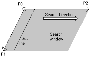
Example: Finding an edge pair within an Area. Refer Edge example application.
Once the projection has been calculated, it is possible to commence edge detection. An edge is defined as a transition from black to white (positive edge) or white to black (negative edge). Three methods of detection are used in the CVB Edge Tool.
See also the Edge example application.
In the Edge Tool we use the simplest and fastest method to calculate the position of an edge in the subpixel range: linear interpolation. This enables the position of an edge to be determined to a precision of approximately 1/10th of a pixel.
The quality of the framegrabber used is of importance here. If possible, the images should be recorded using a pixel-synchronous framegrabber. This type of synchronization precludes PLL errors.
The functions using the threshold and the contrast method are implemented with and without support for subpixeling. Functions using the optimzed method are always returning edge locations with subpixel accuracy.
Within the edge detection functions it is possible to use either a
All of them are able to find the first edge, a pair of edges or all edges within a given image.
With this method, the first point within the normalized projection whose value lies above or below a given threshold is sought. The following diagrams illustrate this procedure:
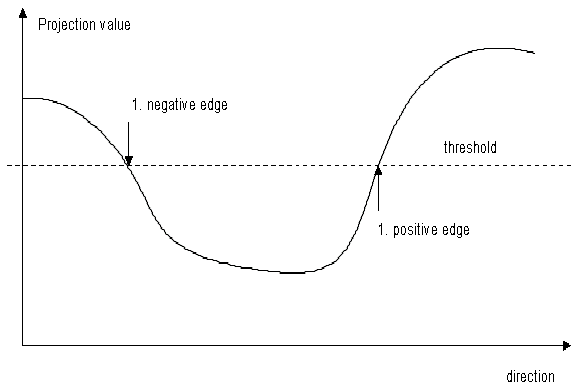
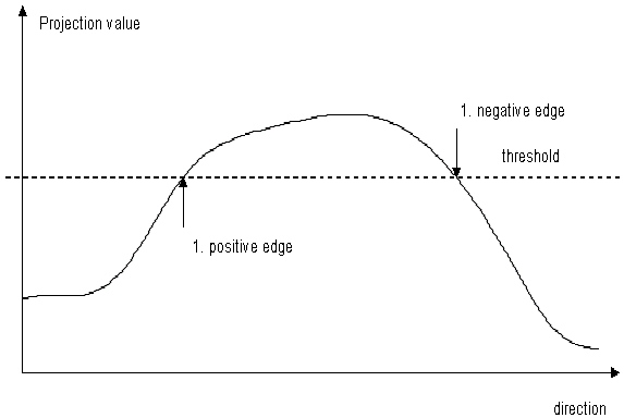
Detection using the threshold method is very simple and quick. The disadvantage is that it is greatly dependent on the lighting used. This method should be used with constant lighting only. However, the method is particularly advantageous if a backlight source is used.
With the contrast method, detection is not performed directly using the projection, but with its first derivation. An edge is therefore detected by means of the difference between two neighboring projection values. With reference to the graphic, this means that the gradient of the curve must assume a minimum (negative edge) or maximum (positive edge) value. The image below shows a simple object:

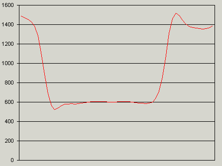
This graph shows the projection data of the area marked in the image above:
The next graph visualizes the projection data (red) and its first derivation (blue). Notice that we introduce a second y-axis displayed on the right side of the graphic:
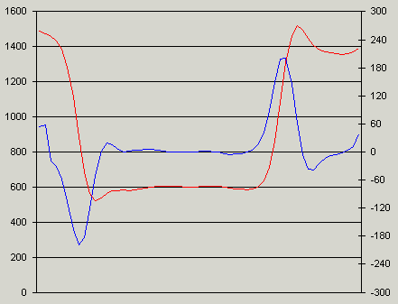
The contrast based method uses the same algorithms as we use in the threshold method, but instead of using the projection data, the contrast method uses the first derivation of the projection. The functions return the positions were the first derivation crosses the specified threshold.
The advantage of this method is that it is (relatively) independent of the lighting used. When the lighting changes, this will simply cause an offset in the projection values, but the contrast will largely remain stable. The calculations required with this method are more complex than with a simple threshold method, so this variant does require slightly more time. Always use this method whenever it is impossible to ensure constant lighting. Note that, with this method, the threshold values are much lower than the actual gray value, since they do not describe the gray value itself, but rather gray value changes.
As we learned in the previous chapter the contrast method returns the position where the first derivation crosses the specified threshold level.
It's obvious that this position does not refer to the real edge position. The real edge position is defined as the point where the curve changes its direction from left to right or from right to left. Zerocrossings in the second derivation are exactly what we want to detect.
The image below shows again the simple object and the first graph visualizes the projection data (red) and its first derivation (blue). Notice that we again use a second y-axis to display the first derivation:


Now lets take a look to the second derivation. It's displayed below as a green line:
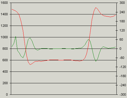
As you can see, the positions where the green line (second derivation) crosses 0, refer to the positions where the red line (projection data) changes it's direction. The functions using this method perform the following steps:
As you can see the functions return the position of the edges with a pretty high accuracy. On the other hand it performs a lot of operations on the image data as well as on the projection data and it's therefore slower than the other two methods.
Use this function type if you need high accuracy. If speed is more important in your application use the threshold functions. A good compromise between speed and accuracy are the contrast functions. They are pretty fast and accurate.
This example demonstrates nearly all features of the Edge library. Notice how the area effects the scan direction. The first Edge P(white) is a positive Edge and P(red) is a negative Edge.
Find more examples in the Tutorial directory under CVBTutorial\Edge.