
Common Vision Blox Tool
 C-Style |  C++ |  .Net API (C#, VB, F#) |  Python |
| SF.dll | Cvb::ShapeFinder2 | Stemmer.Cvb.ShapeFinder2 | cvb.shapefinder2 |
Shape recognition - simple, fast and flexible
ShapeFinder and ShapeFinder2 are search tools to find previously trained objects in newly acquired images.
ShapeFinder2 returns the object location with subpixel accuracy as well as the rotation angle and the scaling of the object found. Of course it also returns a quality measure for each object found. One particular feature of the software is it's tolerance to changes in the object that may appear in production lines such as:
Both tools have also the ability to recognize and measure rotations and scales. It can searched for multiple objects within one image. Setting parameters the user has the choice between an extremely fast or a slightly slower but more accurate and more reliable recognition.
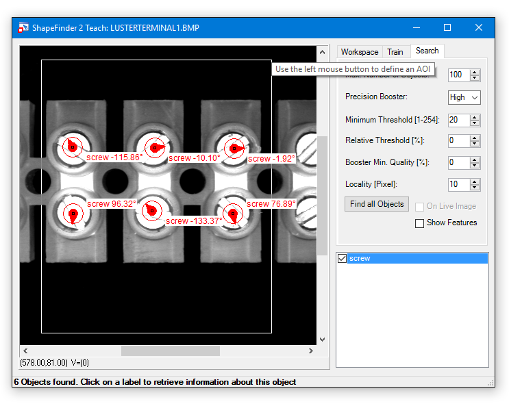
Image Processing Tool for Shape recognition
This part of the documentation is intended to give a detailed explanation of ShapeFinder principles and algorithms,
The purpose of the various API functions and their (sometimes unexpected) behaviour. This is valid for ShapeFinder and ShapeFinder2 usage. Find the ShapeFinder2 enhancements described in chapter ShapeFinder2 Theory of Operation.
In this section we explain how ShapeFinder finds and represents shapes in images.
Instead of the word 'shape' we might also use 'pattern' or 'object', but as ShapeFinder relies mainly on the geometric information of edges, 'shape' seems most appropriate. Hence the tool name we will nevertheless use the other terms freely in this document.
The rather simple algorithm of ShapeFinder is designed following the principles of the generalized Hough transformation, and we can make no great claims to originality for our invention.
When training a pattern from an image we must specify
In the API function CreateSFFromImage the parameters Image and Index specify the training image and the corresponding colour plane, MX and MY correspond to the pattern position, and FWL, FWT, FWR, FWB describe the feature window rectangle. Threshold is the minimum gradient slope as discussed above.
When the function executes, it scans the feature window for pixels, where the gradient slope is larger or equal to the threshold Θ, and for every such pixel records the following:
The list L, of all these quadruplets of vector components and gradients (dx, dy, α, σ), is the complete data set that ShapeFinder uses to find the pattern. We call this list L the feature list of the pattern and the individual quadruplets features.

The schematic image above attempts to illustrate the recognition relevant properties (dx,dy,a) of a feature.
The Hough transformation finds a pattern solely on the basis of gradients (edges, contrasts or inhomogeneities) in an image. These gradients correspond to pixels in whose neighbourhood the images gray values change sufficiently. Points in an image, in whose neighbourhoods the gray values are approximately constant are ignored by the algorithm. The precise meaning of the words 'sufficiently' and 'approximately' will be clarified below. The gray value-gradient at a pixel has two properties: Direction and slope.
The direction is an angle and might be given in degrees or radian.
It will however become clear in section "Directional Quantization and Angular Tolerance", that we have to quantize these angles rather roughly.
We will use integral units of 1.40625° per unit. This seemingly odd quantity is chosen so that a full 360° corresponds to 256 units, which is obviously of computational convenience. The slope is a positive number of gray values per pixel. A slope of 30 means that the image gray values increase by 30 units over the distance of one pixel.
In chapter "Gradients" the properties of the gradient types used by ShapeFinder are discussed in more detail. We can now define the words 'approximately' and 'sufficiently' more precise:
ShapeFinder considers only pixels with gradients whose slope is above or equal to a user specified minimum or threshold Θ. From all of these pixels the position and gradient orientation information is collected as feature information. All other image information is discarded.
The slope threshold Θ is a system property chosen by the user. The values to choose depend on the nature of the pattern to be trained, and on the contrasts expected in the image.
When searching an image rectangle for a pattern, ShapeFinder uses the feature list to compute a numerical similarity or quality for each point in the search-rectangle.
The pattern is most likely be at the point where this quality is at a maximum. A corresponding quality-valued image (the so called accumulator A) is returned to the user for more sophisticated post-processing.
ShapeFinder's recognition technique is essentially the counting of matching features. The definition of the quality A(x, y) for a given image point (x, y) in the search-rectangle is very simple:
A(x, y) is the number of all those members (dx, dy, α, σ) of the feature list L such that:
The positions (x+dx, y+dy) are just displacements of the pattern features at (dx, dy), to the image position (x, y). The displacement corresponds to moving a pattern template to the position (x, y) in the image. After the displacement, the coinciding gradient directions are counted. Evidently the patterns σ-values are not used in the recognition process.
We have not yet clarified what is meant by coinciding gradient directions. If we measured angles as real numbers, clearly the tiniest amount of noise would threaten to destroy equality, and most accumulator values would be zero or near zero.
In any case, this is an insufficient basis for making an accurate decision. For this reason we have divided the full 360° circle into 256 sections, making equality of the values of angles more likely using coarser units of 1.40625°.
Nevertheless, as noise increases, equality of angles can again become rare. It would at first appear that even coarser units of angular measurement would help. As it turns out this is not really a good solution because of the noise susceptibility near the quantization boundaries.
Instead we have retained the 256 possible angles and opted for a more stable approach, introducing another global parameter called the angular tolerance AT, which controls the definition of coinciding directions:
Two angles a and b coincide if:
min{|(α-β) mod 256|, |(β-α) mod 256|} ≤ AT.
This cumbersome expression comes from the modular arithmetic for angles and really means | α-β | ≤ AT. So angles are regarded as coinciding if they differ by no more than the angular tolerance AT. If AT=0 then angles coincide if and only if they are equal.
It is important for the efficiency of the ShapeFinder search algorithm, that the angular tolerance can be absorbed in the construction of a new feature list.
Suppose that for a given original feature list L, we construct a second list LAT such that for every one record (dx, dy, α, σ) of L we include in LAT all records (dx, dy, α+γ, σ), where γ ranges from -AT to AT (always mod 256).
Then working with L and a positive value of AT is equivalent to working with LAT and an angular tolerance of AT=0. These two approaches result in the same quality function A(x, y).
Working with equality instead of tolerances is essential for the efficient implementation of ShapeFinder as shown below. We therefore generally maintain two lists for every model: An original list L obtained by training from an image, or some synthetic operation, and a second list LAT, which absorbs the angular tolerance parameter.
The second list is constructed automatically whenever the first list is created (all CreateSF-functions), and whenever the angular tolerance parameter is modified using the function SetSFAngularTolerance.
It will become clear from the definition of the search algorithm that increasing the angular tolerance, while improving the robustness, also decreases the execution speed of a search. The list LAT is after all (2AT+1) times as long as the list L.
The primary task of the search algorithm is to compute the quality values A(x, y) for every point (x, y) in the search area. Given the definitions above, the most straightforward and conceptually simple way to do this would be to:
This approach involves a large number of computations. The order is the size of the search area, multiplied with the number of list entries (dx, dy, α) ∈ L. It turns out that it is much faster to compute A(x, y) in a more devious way.
Instead of going over all possible candidate points for the pattern position and then checking the required gradients, we go over all pixels measuring the gradients, and if such a gradient has sufficient slope we increment A(x, y) for all possible candidate points which are compatible with the measured gradient direction.
Specifically the algorithm proceeds as follows.
It is easily seen that the algorithm produces the same values of A(x, y), but that the number of computations will be typically much smaller.
The model information is considered only for those points in the extended search rectangle, where the gradient slope is sufficiently large, and even then only a small subset of LAT is used. To rapidly execute the last two steps it is convenient to reorganize the structure of L.
We use an array of 256 pointers, where the α'th entry points to a sublist containing exactly those vectors (dx,dy,σ) such that (dx, dy, α) ∈ LAT. We then only need to address this array with the measured gradient direction and increment A(x-dx, y-dy) for all the (dx,dy,σ)'s in the resulting list (the gradient slope s has no relevance in the search).
Suppose we want to search for more than one type of pattern class (classes C0, C1, ..., CN-1) in the same image and search area. Having trained N corresponding models M0, M1, ..., MN-1, we could just search the area N times and then compare the N accumulator values A0, A1, ..., AN-1. But then we would have to compute the same gradients N times.
Another, typically faster approach is to compute each gradient only once and then update all accumulators A0, A1, ..., AN-1. The procedure is almost identical to the one described in the previous section, only that we have more than one accumulator, and that for every (dx, dy, α, σ) we also require a class- or accumulator index h, which specifies the accumulator Ah to be incremented.
In this way we arrive at a multi-class representation which is a set of quintuplet features (dx, dy, α, σ, h), where
As pointed out in the previous section it is necessary for an efficient search, that this set is arranged as an array indexed by the gradient angle a.
We thus arrive at the following structure for model-lists (ignoring the distinction between L and LAT, assuming henceforth that LAT is created from L whenever necessary):
Here is an example of how such a list might look:
| α | L(α) |
|---|---|
| 0 | (dx1,dy1,σ1,0), (dx2,dy2,σ2,0), (dx3,dy3,σ3,2) |
| 1 | |
| 2 | (dx4,dy4,σ4,1) |
| ... | ... |
| 255 | (dx5,dy5,σ5,0), (dx6,dy6,σ6,1) |
The collective feature window (FWL, FWT, FWR, FWB) for all the classes contained in such a multiclass model, is computed from the list L as a simple bounding box for all the vectors (dx, dy) in the list. Correspondingly the extended search area (L+FWL, T+FWT, R+FWR, B+FWB) is computed for every given search area (L, T, R, B).
Here is the final definition of the ShapeFinder Search Algorithm:
So far we have talked about gradients, taking for granted the existence of gradient-computing algorithms. This is by no means a trivial problem, and there is a lot of literature dealing with the computation of gradients on a lattice with many different proposals.
The simple pair of partial derivative operators (δ/δx, δ/δy), familiar from elementary calculus for functions defined on a two dimensional continuum, has all the desired properties, but an equivalent pair of operators for the discrete case can only be approximated.
The crux property is isotropy, the ability of the gradient to measure the slope of edges independent of their orientation, and to measure accurately the orientation.
Computation speed is also an important issue. Some proposed gradients compute very fast and have poor isotropy, while others reduce measurement errors at the expense of execution time.
In the design of ShapeFinder we have decided to offer one option from each category (the Roberts and the Optimal Sobel gradient) and leave the choice to the user. A model trained with one type of gradient, however, will always have to be used with the same gradient type.
By the nature of the ShapeFinder algorithm, the contribution of the gradient to execution time becomes relatively small for complex models or multi-class models. In these cases the execution speed of the gradient should not be considered.
Every gradient can be considered as a pair of operators (A,B) which for every image-grayvalue distribution g, and every pixel point (x,y), produces a pair of numbers (a,b) = (Ag(x,y), Bg(x,y)).
Then, the slope of the gradient is defined by |(a,b)| = sqrt(a2+b2), and the direction as arctan(a,b).
Regardless of the type of gradient employed, ShapeFinder computes slope and direction with a lookup table which is programmed during startup of the ShapeFinder library, and addressed with the components (a,b) of the gradient vector.
The operators A and B replace the partial derivatives of the continuous case and should be translation invariant and linear, therefore representable by convolution kernels.
Constant images should result in zero gradients so the kernel sums must be zero. An image rotated by 180° about a pixel should have the negative gradient at this pixel, so the kernels should really be antisymmetric.
Finally the kernel of B should be related to the kernel of A through a 90° rotation.
For practical purposes these kernels should be finite. There is one complication arising from the lattice structure which should be understood by the user:
Suppose that you create a synthetic image by drawing a black line at a 6° angle to the x-axis in a white image. The result with a standard line drawing algorithm will look something like this:

It is clear from looking at this image, that in the middle of one of the horizontal stretches no gradient measurement with kernels of less than 10 pixels diameter can detect the 6° orientation of the line. Every local measurement will return an angle of 0° at these points, with different results near the line-hopping points.
The situation is changed, when the line drawing is carried out with an anti-aliasing interpolation. In this case the gray values in the bottom line increase from one pixel to the next, while those in the line above decrease. The information on the orientation of the line is still locally available, and a localized measurement is possible. This problem is not academic, but arises whenever you rotate a rigid object with good contrasts by a small angle.
If your optical focus is better than the resolution of your camera target, you violate the essential assumptions of the sampling theorem corresponding to the first case above, and cause yourself a lot of trouble.
The same happens when you arrive at gray value saturation because your contrasts are too large. There is a psychological difficulty because humans tend to associate good optical focus and high contrasts with good image quality, ignoring the subtle implications of lattice quantization in digital imaging.
Here are some general hints to get good results with ShapeFinder:
This is the fast solution. The operators A and B are given by 2x2 convolution kernels:
 ,
,
The components of these gradients can be computed very quickly and it will never obliterate any high resolution details in the image. The derivative operators, instead of operating along the usual coordinate axes, work along the diagonals resulting in a gradient vector rotated by 45° from the usually expected direction. This causes no problems in the context of ShapeFinder, where it is ensured that models trained with the Roberts gradient will only be used with the Roberts gradient.
The dynamic range of both operators on an 8-bit image is from -255 to 255 each, so that 18 bits are required to represent the gradient vector without loss of information.
This means that 262144 entries are needed for the lookup table for gradient slopes and directions. Since each entry contains an 8-bit slope and direction information, we require 524288 bytes of memory for the lookup table. Programming this table takes time and is executed only once, when the ShapeFinder library is loaded.
The Roberts gradient has some disadvantages:
Use the Roberts gradient, whenever you:
The operators A and B are given by 3x3 convolution kernels:

This gradient is optimal with respect to directional measurements, given the 3x3 kernels.
For wavenumbers below 0,5 the directional error remains below 0,7° [Jähne]. It destroys highfrequency information, in particular it annihilates the Nyquist frequency (alternating pixels). The optimised Sobel gradient requires more computation time than the Roberts gradient. This is generally irrelevant in the case of very complex models or multi-class models.
Use the optimised Sobel gradient whenever you:
In this section we explain how ShapeFinder allows for the combination of models to create new models with new properties.
This can be done either by superposition giving rise to new models with enhanced recognition properties, or by concatenation to create multi-class models capable of recognising different pattern types, allowing ShapeFinder to be used for simple OCR applications, such as the reading of numerals.
As explained in section "Multi-Class Models and Searching" the model information is essentially contained in a list L, of records or quintuplet features (dx, dy, α, σ, h) describing the displacement to the pattern position, the gradient direction, the gradient slope and the class- or accumulator index h respectively.
For the purposes of the search algorithm this list is conveniently arranged as an array indexed by the gradient angle α.
To understand the different methods of model combinations we go one step further, and imagine L as a two dimensional array indexed by α and h. Then an entry L(α,h) of this array is a pointer to a list of all those (dx, dy, σ) such that (dx, dy, α, σ, h) is in the original list L. This is only a conceptual step. Here is how such an array can be visualized:

The green stacks correspond to the lists of (dx, dy, σ). Of course some of these may be empty. When a model has been trained, only the value h=0 exists, so there would be only the leftmost column in the above array. The diagram corresponds to a case of three classes.
This is the basis of training for multiclass models. In this case the representation of the pattern classes in model M1 remain unchanged. For every class index of model M2 a new class index is created and appended to model M1. The following diagram illustrates the operation:

This operation is carried out by the ShapeFinder API function ConcatenateSF. A simple method to train a model for the characters '0', '1', '2', ... '9' would thus proceed as follows:
The function CreateRSymmetricSF also uses the concatenation function in a more complicated way to create a rotation invariant model as shown in section "Rotation Symmetry".
This method can be used to make the model more robust and is equivalent to the addition of accumulators. From M1 and M2 it creates a model collecting all the features of both without the creation of new class indices for the previous members of M2. The following diagram illustrates the operation:

This is carried out with the ShapeFinder API function MergeSF. An important example is the case of partial contrast reversal. The ShapeFinder API contains a function CreateContrastReversedSF, which given an input model for some kind of pattern, constructs a model capable of recognizing the negative pattern.
There is no great magic to this function: A negative image just has gradients rotated by 180°, so all CreateContrastReversedSF needs to do is to add 128 (modulo 256) to all α's in the input list. It now happens frequently in applications, that an image acquired from a shiny surface suffers from partial contrast reversal: The image is positive in one area and negative in another, the problem can even divide a moderately extended pattern. With ShapeFinder you can solve this problem by:
An equivalent but more time- and memory consuming result would be obtained by using ConcatenateSF on the two models and adding the two accumulators A0 and A1 after every search.
In cases where the ideal form of a pattern is not available in images, ShapeFinder allows the definition of models in terms some elementary graphic operations, the drawing of line segments. Circles, the conceptual starting point for the 'classical' generalized Hough transformation are also supported.
The model creation primitives described below would not be very useful if it wasn't possible to geometrically translate primitives using the API function CreateTranslatedSF and to combine them using the function MergeSF described above.
The function CreateTranslatedSF simply adds a specified two dimensional offset to all the dx, dy in the model, essentially effecting a change in pattern origin.
In section 'Graphics' we will show an example, how a model for a rectangle of specified dimensions can be created.
The algorithm of ShapeFinder is most easily understood in the context of circles.
Assume we want to recognize white-on-black circles with given radius R. We scan the image and when we come across a sufficiently large gradient, we pause and ask ourselves:
'Can this be part of a circle, and if so where might its centre be?'
The circle boundary assumes all conceivable orientations so the answer to the first part of the question is always yes. But in the case considered, the gradients at the boundary edge always point to the centre. So the centre is in the direction of the gradient, a distance of R units away.
This is where we have to increment the accumulator, which counts or 'accumulates' the number of boundary points the circle would have if its centre was at the position of that particular accumulator cell.

The ShapeFinder API function CreateSFCircle creates a model for the recognition of black on white circles of specified radius. The corresponding feature list has exactly one entry for each angle a.
Use the function CreateContrastReversedSF to make a model for white on black circles and the merging function as in section 'Superposition and Merging of Models' to create a model for circles of arbitrary contrast.
The reader familiar with the Hough transformation for circles will remember that there is a trick for the detection of circles with radius in a larger range of values.
Instead of incrementing the accumulator only at the position of distance R from the detected gradient, it will be incremented along a line segment in the direction of the gradient.
The distances where the segment starts and ends correspond to the boundaries of the possible values of the radius.
The user of ShapeFinder will recognize that this technique is equivalent to the behaviour of a model obtained by merging a collection of models defined with CreateSFCircle and R ranging over a set of value. So the same technique can be used with ShapeFinder. But one can do even more: Using the concatenation function ConcatenateSF on several such models corresponding to subranges for the radius, one obtains a multi-class model yielding additional information on the size of the circles detected. An additional benefit is the improved signal-to-noise ratio at the penalty of greater memory requirements.
This is another simple synthetically generated model for the detection of straight edge segments of specified orientation and length. This is a local model not to be confused with the global technique of the Hough transformation used to detect straight lines.
The models created by the ShapeFinder API function CreateSFSegment have their pattern origin at the segment centre. The model detects edge segments of specified length l, and orientation. As with circles, this case also illustrates the principle of the ShapeFinder algorithm.
Again we imagine scanning the image and coming to a gradient with sufficient slope, pause and ask:
'Can this be part of the sought edge segment, and if so, where might its centre be?' 'If this pixel is part of the sought edge segment, where might its centre be?'
There are two cases. If the gradient direction does not correspond (within AT) to the orientation of the edge we seek, the answer to the first question is negative. Thus the feature list L(α) must be empty for all a which are incompatible with the desired edge orientation.
On the other hand, if the gradient has the right direction, the centre might be anywhere along a line segment of length l perpendicular to the gradient a. In this case the accumulator must be incremented along this entire line, and L(α) is a list with l elements (at least in principle, ignoring aliasing problems).

The API function CreateSFSegment takes the orientation angle and the length as arguments. An orientation of 0° corresponds to a gradient of 90°, which is a horizontal edge with low gray values below and high gray values above.
The synthetic models for edge segments and the API functions CreateTranslatedSF and MergeSF make it possible to create synthetic models for arbitrary objects, composed of a finite number of edge segments. What needs to be done is:
The following program fragment, written in Pascal, demonstrates the creation of a synthetic model for the detection of 30x20 pixel black rectangles. Thr and Gtp stand for threshold and gradient type (Roberts or optimised Sobel). Temp, Temp2, LeftEdge, TopEdge, RightEdge and the result Rectangle are pointer variables.
In this section we describe the technique of simple geometric transformations of models and discuss some applications, in particular the creation of rotation invariant models.
Linear transformations of the plane are representable as 2x2 matrices:

The first column gives the components of the vector we get, when we transform the unit vector in the x-direction. The second column is the transformation output for the unit vector in the y-direction. For other input vectors the transformation is defined by linearity.
Important special cases are the rotation matrices:

which rotate a vector by an angle α (in radian), and the scalings:

which scale by a factor s.
All these transformations can be combined and there are many others, such as mirror reflections and shearings, included among the 2x2 matrices.
Using the ShapeFinder API function CreateTransformedSF, all these matrices can be applied to ShapeFinder models thus creating new model capable of the detection of correspondingly transformed shapes.
CreateTransformedSF works by transforming all the members ( dx, dy, α, σ, h ) in the feature list separately, using the results for the feature list of the transformed model. Only the displacement (dx,dy) and the gradient direction a need to be considered. σ and h carry no geometrical information. (dx,dy) transforms just as any vector is transformed by a matrix.
The problem with this operation is that the result has to be truncated to integral values because of the discrete nature of image and accumulator, there is no way around it. For this reason you can sometimes see 'holes', when you transformed a model with a matrix and look at the result, using the GetSFImage function.
The gradient direction α is transformed by first constructing a unit vector pointing in the direction of α, then transforming this vector with the given matrix, and finally measuring the direction of the resulting vector.
Of course this procedure will give the desired results only if the transformed gradients in an untransformed image are the same as the untransformed gradients in the transformed image.
If we measure a 0° gradient direction in the original image and a 6° gradient direction in an image rotated by 12°, things will not work properly. This is when we require good isotropy properties of the gradient measurement.
The isotropy of the Roberts gradient isn't all that good, but the error of the optimised Sobel gradient is well within our limit of angle quantization, at least for reasonably low wave numbers (see section 'The Optimised Sobel Gradient').
This is why we recommend the Sobel gradient whenever you intend to use geometric transformations on models.
Geometric transformations of models can be used together with the merging and concatenation functions to arrive at a rotation invariant pattern model. The idea is very simple:
We create one model from training (using the Sobel gradient), use CreateTransformedSF to rotate it sufficiently close to every possible rotation angle and merge and/or concatenate the models together.
When we say 'sufficiently', we mean that the recognition with ShapeFinder works well over a corresponding range of angles. The maximum tolerable range depends on the type of pattern trained, and on the minimum signal to noise ratio which you are willing to accept.
You can determine it experimentally by training the pattern and rotating the image until the signal to noise ratio (quotient of accumulator maximum at pattern position to next largest maximum) drops below the acceptable level.
In practice 5° is a safe value, so if you cover the circle with 36 rotated models, to always stay within 5° of one you should get reasonable recognition results.
Nevertheless this might fail for a very extended and complex pattern, while it might be an overkill for something very coarse or simple. A pattern which is itself rotation invariant such as a circle, needs only one model and considerable simplifications are possible for patterns which are invariant under some subset of rotations, such as squares or any regular polygons.
The next question is whether to merge or to concatenate the models. It turns out that merging too many very different models together, doesn't work very well. The features begin to combine in many ways which are inconsistent with the original pattern in any of its rotation states. Thus one feature of the original pattern can combine with another of the 60° rotated pattern and another of the 120° rotated pattern.
In this way a significant contribution to the accumulator can arise from a phantom pattern which has nothing to do with the shape originally sought, and the signal to noise ratio becomes very low up to the point where recognition is impossible.
Concatenation is generally better, in addition to the improved signal to noise ratio there is the benefit of coarse information on the rotation of the object which has been detected.
The disadvantage of concatenation lies in the large amounts of memory required for the accumulators. Each accumulator cell requires two bytes of memory otherwise numeric overflows would occur very frequently. So for a 500K image, 36 accumulators need 36 megabytes of memory so your computer has to be well equipped.
As so often, a compromise is best. Use the merging for similar angles and concatenate the resulting models. The phantom pattern created by the merging of similar models is not too unlike the pattern in question and often represents realistic deformations.
You could program the creation of rotationally symmetric models using the other API functions, but we have saved you this work by including the function CreateRSymmetricSF.
The function covers a range of angles specified by the parameters Alpha0 and Alpha1, corresponding to the start and end point of this range. This range of angles is subdivided into NAccus equally sized cells, corresponding to the number of accumulators used. (Alpha1-Alpha0)/(2NAccus) is thus the maximum error of the implied measurement of rotation angle.
For each of these cells, models are created which are then concatenated. The models corresponding to the cells are created by subdividing the cell into NPerAccu subcells, creating a submodel for the central angle of this subcell by rotation of the original input model, and merging the submodels together.
(Alpha1-Alpha0)/(NAccus*NPerAccu) is then the spacing of all submodels on the angular range.

The above diagram illustrates this division corresponding to a call with Alpha0 = 45, Alpha1 = 225, NAccus = 4 and NPerAccu = 3. The submodels are spaced at 15° intervals, there are four accumulators (I - IV) and the precision of angular measurement is up to 22,5°.
In this chapter we explain some of the more subtle properties of ShapeFinder. In particular we discuss the nature of the accumulator values, and some cases where ShapeFinder might fail to behave as expected.
The accumulator, as output by ShapeFinders SFSearch function, has the same dimensions as the input image, and we can identify points of the accumulator with points in the input image.
Ignoring the boundary effects of the search area, a search of a shifted input image results in a correspondingly shifted accumulator. So ShapeFinder's search acts like a translation invariant, nonlinear filter, the output of which can again be subjected to the techniques of image processing.
The only image processing which ShapeFinder's search function applies to the output, is the computation of the global maximum. A very simple improvement is furnished by applying the CVB function FindMaxima to the accumulator.
The result is a list of local maxima, corresponding to the various local maxima. This list, the output of the simple 'SearchAll' function thus constructed, can be sorted in a variety of different ways as documented in the CVB manual.
It is the hope of ShapeFinder's users as well as of its designers, that the accumulator values provide some kind of reliable quality measure for the occurrence of a pattern within an image, a quality related to the intuitive idea of similarity.
This hope is largely justified, but not completely, and in the following we discuss some of the more important case of paradoxical behaviour which you might run into.
To facilitate the discussion, lets assume that we are dealing only with a single class model and that we search an image, of which we know by some other means that it contains the pattern exactly once and at some known position.
The accumulator value at any point (x,y), counts the number of features ( dx, dy, α ) in the feature list L, which correspond to points (x+dx,y+dy) in the feature window with gradients matching α.
If the point happens to be the pattern position, and if the pattern in the image is identical to the pattern from which the model was trained, the result will be total number of features in the feature list because every feature will match.
So this number |L| , which is the maximum value possible will be attained when the pattern is an exact match, and the accumulator values cannot be greater in any other case. This partly justifies the use of the accumulator value computed by ShapeFinder's search function.
If we decrease the image contrast some features will cease to match, because the corresponding gradients will drop below the threshold Θ. But this is a very normal and tolerable behaviour, the same happens when portions of the pattern are hidden.
In this case it takes a lot of hiding for ShapeFinder to loose the pattern, and the software appears spectacularly robust to people unfamiliar with the underlying algorithm.
These are good sides. Now we come to the problems: The first problem lies in the fundamental fact that ShapeFinder always requires the presence, but never the absence of gradients. This is immediately clear from the definition of the algorithm, but it can produce paradoxical results. If you train this pattern

and run SFSearch on these two images

the right will return a higher and near maximum quality, even though it is less similar to the human eye. The remedy is conceptually simple but takes a little bit of execution time, a little bit more programming effort and some extra software:
Run the 'SearchAll', as explained above, over the accumulator and use a normalized gray value correlation to determine a reliable quality measure for the strongest accumulator maxima. The correlation will take little time because it needs to be computed a few times.
While the first problem was of the 'false positive' type (accumulator values too high), the second problem is with 'false negatives', where the pattern instance should really be accepted but is likely to be rejected because the accumulator values are too low.
Suppose we have trained a simple but very extended pattern, extended in the sense that the features are far away from the pattern position, say about one hundred pixels.
Now we rotate this object by a minute angle of 0,6 degrees and we notice a dramatic decrease in accumulator values.
Consider a feature at a distance of 100 pixels from the pattern origin. Rotating about the pattern origin by 0,6 degrees has the effect of translating a point at a distance of 100 pixels by approximately one pixel to the side, the gradient direction however will in most cases be unaffected because of the angle quantization in steps of 1.40625°.
This means that the corresponding gradient of the rotated pattern will make no contribution to the accumulator at the pattern position (hence the decrease), but it will increment the accumulator one pixel off to the side.
There are several conclusions to be drawn.
In essence the last idea is related to the lowpass-filter idea above, but it is much cruder and immediately halves the accuracy of position information. But there is the benefit of increased robustness without any loss in execution speed.
There is a tremendous benefit in memory critical situations (e.g. rotation invariance), because the downscaled accumulator has only a quarter of the pixels. This can even lead to a slightly increased execution speed because of increasing efficiency in cache utilization.
For these reasons we have included the parameter Pitch in the API function SFSearch.
Pitch is just a downscaling factor for the accumulator.
For the convenience of the user the downscaling is completely hidden and carried out within CVB's VPA-table structures.
Up to this point the number of features representing a given pattern class is a consequence of the trained image, the gradient slope threshold Θ, and the various subsequent merging operations.
There are two important reasons why we would like to directly control the number of features of an already existing model and class, in the sense of setting it to some defined value.
Assume now that in some given model there are Nh features for each class index h, that is: With a given h there are Nhh quintuplets (dx,dy,α,σ,h) in the feature list.
Suppose that we wish to enforce the feature number M > 0 for each class. Now for each h there are three cases:
This is what the ShapeFinder API function CreateSelectedSF does. To understand how it is really done we must still outline what criteria are used to determine which features are better and which are worse.
There are three criteria, one positive and two negative:
In this section we summarize the properties of the four most important parameters in a table:
| Threshold | Angle Tolerance | Pitch | Gradient Type | |
|---|---|---|---|---|
| Explained in section | 'Counting Contrasts' | 'Directional Quantization and Angular Tolerance' | 'Properties of the Accumulator' | 'Gradients' |
| Purpose | select largest image contrasts for processing | increase robustness of recognition | increase robustness of recognition and save memory | define contrast measurements |
| Value range | 1..255 | 0..16 | 1..3 |
|
| Typical | 25 | 1 | 1 | X |
| Effect of increasing value | fewer features, recognition down, speed up | recognition up, speed down | recognition up, speed slightly up, accuracy down, memory use down | Opt. Sobel: slower, more accurate, good transformation properties |
| Effect of decreasing value | more features, recognition up (up to a point), speed down | recognition down, speed up | recognition down, speed slightly down, accuracy up, memory use up | Roberts: fast, noise susceptible, poor transformation properties |
| Value saved on disk | yes | yes | no (parameter of SFSearch) | Yes |
| Can always be modifies | yes, but careful when modifying | yes | yes | no, fixed property of Model |
For starting new projects please use Shapefinder2 functionality. In special cases Shapefinder can be an option. But this should be discussed with our technical support team.
If a Shapefinder user is missing the functionality to generate circles in Shapefinder2 it is still better to use Shapefinder2. To teach a circle you can create a synthetic image in your favorite image editing program. e.g. a white circle on a black background. Then you can use this synthetic image to teach Shapefinder2.
We outline here the basics of Shapefinder's enhanced functionality. The reader is also referred to the corresponding chapter Theory of Operation in the general Shapefinder manual.
To sketch the operation of ShapeFinder2 it is helpful to introduce the concept of a generalized position of a pattern. This incorporates the position of one or more pattern within an image, but may also contain the rotation and/or orientation of the pattern relative to its trained instance, if so desired by the user. The generalized position is therefore described by a five-dimensional vector (Q, X,Y,A,S). See datatype TSFSolution. If no rotation is to be measured A is set to 0, if no scale-measurement is desired S is set to 1.
The execution of a search function with SF2 is carried out in three steps:
The preliminary search is carried out with the ShapeFinder-algorithm (Hough-transform as described in the documentation for the previous version) at a reduced resolution.
The resolution used (downscaling by factors of 1,2,4,8,…) is determined in the training process, during execution of the function CreateSF2. The exponent i of such a scale 2i is returned in the CoarseScale-parameter by the function GetSF2Features. The geometrical positions of the features used in the preliminary search are returned in the CoarseFeatures-pixel-list parameter of the same function.
During training these features are concatenated with appropriately rotated and scaled clones to a ShapeFinder-model appropriate for searches in the reduced scale. This model is then used to scan the image and to write to a four-dimensional accumulator/histogram H(X,Y,A,S). Intuitively H(X,Y,A,S) is proportional to the supporting evidence that there is a pattern at position (X,Y) in rotation state A and scale S. After the image scan a list L of local evidence-maxima is extracted from the accumulator. This process and the definition of local maxima is controlled by the TSearchAllParams-structure governing the search.
If the Precision parameter in the TSearchAllParams-structure governing the search is set to 0, the search is terminated after the preliminary search, resulting in quickest execution but also lowest accuracy, with errors of up to several pixels in positioning and several degrees of rotation and considerable scale percentages, all depending on the pattern in question and the coarse scale employed.
In this case L corresponds to the Solutions-parameter returned by the SF2Search-function and the Qi correspond to the accumulator values at the generalized positions or the local maxima.
Now every generalized position (Xi, Yi, Ai, Si) returned by the preliminary search is used as a starting point for a correlation based hill-climbing algorithm, choosing successive points in a sequence of generalized sub-pixel neighbourhoods to improve the match of the appropriately shifted, rotated and scaled image to the trained pattern, until no further improvements are possible at a step-size of 128-1 pixels.
In this way a second list L' is generated from the data in the first list, and the Qi now correspond to the correlation values at the 'hill-tops'.
Although the search is a sub-pixel algorithm, it is still implemented in the coarse-grained (low resolution) image, using for the determination of the correlation the same coarse grained features as before, so that the resulting measurement is accurate only up to a rather large fraction of a pixel/degree (depending of pattern and CoarseScale), which is what happens if the Precision parameter in the TSearchAllParams-structure was set to 1.
If the Precision parameter is set to 2 a final search is used to obtain results of the highest accuracy. The method (correlation-hill-climbing) is essentially the same as in the second step.
The only differences being that now the output of the second step is used as input, and that the algorithm is applied to the original (maximal) resolution of trained pattern and image.
The geometrical positions of the corresponding features for the correlation match are returned in the FineFeatures-pixel-list parameter of the function GetSF2Features.
ShapeFinder uses centred pixel-coordinates. This means that an integral coordinate pair (X, Y) refers to the position at the centre of the pixel at column X and scan-line Y in an image.
The centre of the leftmost-topmost pixel has the coordinates (0, 0) - in contrast to other software packages, where it would have the coordinates (0.5, 0.5). Its upper left corner has the coordinates (-0.5, -0.5).
ShapeFinder2 is shipped with an easy to use Teach application which is also available in VB.NET source code. It supports the following features:
Details regarding the Shapefinder 2 Teach functions are available in the chapter ShapeFinder Library-ShapeFinder2-Teach functions. For an example description how to use Shapefinder2 please have a look at the Shapefinder2 Tutorial.
A ShapeFinder2 Workspace is one or more
Main task of this tab is to open an image via Open Image or Paste Image buttons. For sure Open Image allows to open an image from file or from any image acquisition device like a frame grabber or camera.
Starting with a new Shapefinder project, creating a model or classifier, it is very useful to save the workspace. You are able to reproduce and see all parameters and the images created. This is also a valuable information for support issues.
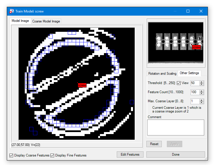
The train tab provides all functionality around a driver model ( *.sf2). Select Add New Model or Open Model. Select the Object Position and the AOI with left Mouse button.
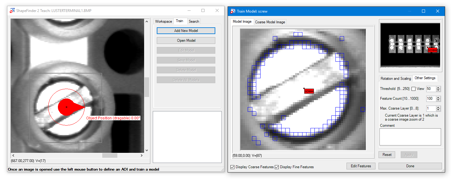
Edit Model - Rotation and Scaling, Other Settings:
| Min / Max Rotation | Define possible minimum and maximum rotation in degree.
|
| Min / Max Scaling | Define possible min and max rotation in percent.
|
| Threshold | Setup Edge Strength.
|
| Feature Count | Define number of features being used.
|
| Max Coarse Layer | Defines the maximum zoom layer used in the preliminary search.
|

Button Edit Features:
The Edit Features dialog offers the possibility to mark so called "don't care regions". If there are parts in the Model Image which are not part of the object please erase the from the model using the tools here like Draw Rectangle. They are marked blue in the Model Image.

Finalize with Apply button and Done.
The search tab allows to test the created model (*.sf2) with all available parameters.
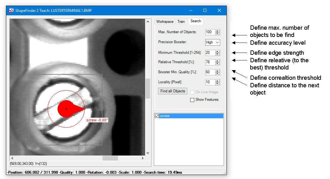
Options for Precision Booster:
Locality:
The locality refers to the center points of the found objects. But the distance is not the euclidean distance. The x and y components are evaluated separately. If e.g. the euclidean distance of two center points is 57 pixels and the angle is about 45° the X and Y distance is about 40 pixels respectively. Thus the locality must be below 40.

Please click on the label of one object to retrieve information about other output parameters like position, quality, rotation, scale factor and processing time:

The Common Vision ShapeFinder2 Search Control provides easy access to the ShapeFinder2 search functions within the ShapeFinder library.
When the Common Vision ShapeFinder2 Search Control has been integrated in a project, a ShapeFinder2Search object can be inserted in your own application via the following icon:
The Control uses the ShapeFinder library to provide an easy interface to the library for all supported compilers. The control provides functions to load a ShapeFinder2 classifier that was created using the ShapeFinder2 teach program (LoadClassifier and LoadClassifierByDialog methods). Or by using the teach functions of the ShapeFinder library (in this case you simply pass the classifier via the CLF property).
All search parameters of the library are mapped to properties of the control.
All these properties are read only. The parameters of the control can be defined interactively using the property page.
The installation of ShapeFinder includes a number of tutorial programs available in source code for different compilers.
Example: C++ Builder demo with Screws
All the screws are found and marked with a label showing the quality and the angle of the found screws. The search result depends on the threshold specified in the example. (Q)uality and (A)ngle are displayed.

This tutorial shows how to use ShapeFinder2 by doing a step by step example with VB.Net ShapeFinder2 Teach Example under: %CVB%Tutorial/ShapeFinder/VB.NET/F2TeachNET. The task is to find the pins of a chip and their orientation.
Finally a few hints on how to use ShapeFinder2 on your own application are given. This tutorial is only an introduction to ShapeFinder2. A detailed description is given here. The images, the sf2-model and workspace are located in the CVB subdirector, %CVB%Tutorial/ShapeFinder/Images/SF2/Chip.
The single steps:


Adding a new model


Here you can see all available model properties and adjust the parameters in the tabs Rotation and Scaling and Other Settings.
Feature Count:
This setting specifies how many features are used to recognize an object. ShapeFinder2 itself determines which features are used.
The tool therefore takes the most noticable parts of the object. In the lower left corner of the window are two checkboxes named Display Coarse Features and Display Fine Features. Activating them shows the features that are used by ShapeFinder2. The coarse features are shown in blue squares and the fine features in red dots.
Threshold:
Go to Other Settings tab. Set the threshold for detecting edges. The threshold value is relative and not an absolute value.
That means an edge is detected when there is a difference of at least the threshold value between the gray value of a pixel and the following neighbor pixel.
Activating the checkbox view shows the image as an edge image. That simplifies the task finding the right setting for the threshold. Just change the threshold when view is checked, to easily recognize which value is suitable for the object to search for.
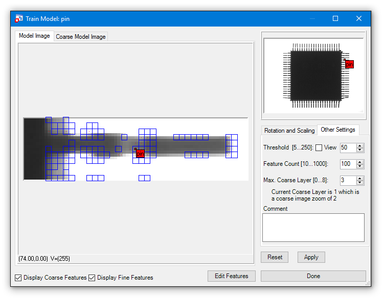
In this case we have first a look at the features which are created.
There are not enough features to describe the shape of the pin, therefore we increase the Feature Count to 200 and show the thresholded image via the View checkbox.
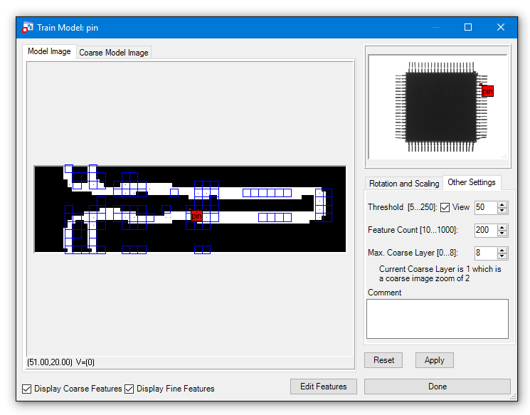
Then we have a look at the parameters from the Rotation and Scaling tab:
Minimum and Maximum Rotation:
Set the minimal and maximal rotation, the objects can have. In the example with the pins a value of +/-180 degrees is to be set to ensure that every possible position of the pins can be recognized.
Minimum and Maximum Scaling:
Set the minimal and maximal scaling, to determine which size difference (relative to the model) the objects can have.
The highest maximum setting is 150 and the lowest minimum setting is 66. As the pins are all of the same size, the default values (100) can be used.

The next steps after pressing Done are
and
Finding the objects
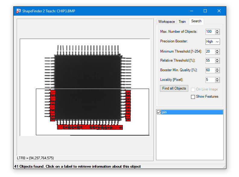

Explanations to the settings are given below.
Max. Number of Objects:
This value defines the maximal number of objects to be found.
Precision Booster:
The accuracy level for the search is defined by this setting.
Minimum Threshold:
Defines the edge strength.
Relative Threshold:
Defines the relative (to the best) threshold.
Example: The model has 100 features defined and the found object matches 50 of these features, the resulting quality is 0.5 (50%).
If the Relative Threshold is set to 60%, the found object will not be labeled. If it is set to 50% or less, the object will be labeled.
This part of the documentation is intended to give you a quick introduction how to...
If you want to search for one or more objects within an image, your system has to "Learn" the pattern in advance. learning is done easily. Use the following steps to test this example: %CVB%Tutorial/ShapeFinder/CSharp/CSShapeFinderOne.

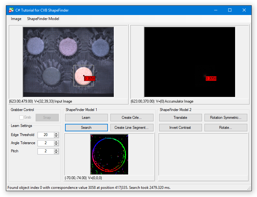
What does the label show?
The label shows:
What does the Accumulator Image show?
(refer to: Example: Search for multiple objects in the same image).
If you search for multiple objects of the same class using ShapeFinder functions, you'll notice, that only the results for the best matching pattern will be reported in most of the samples.
The following steps demonstrate how to search for multiple objects in the same image using ShapeFinder functions. Use the following example: %CVB%Tutorial/ShapeFinder/VC/VCSFSearchAll.
Test this example:
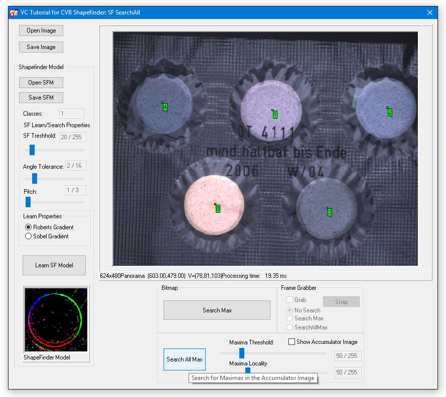
What happened?
Take a look to the output / result of the SFSearch function. You'll notice that the function returns an accumulator image such as this:

After the accumulator image is created ShapeFinder will search for the overall maxima within the image and report it's location and gray value as the object position and quality respectively.
By applying the CVB Image Manager function FindMaxima to the accumulator image we will retrieve a list of local maximas, corresponding to the different object locations. This list can be sorted in a variety of different ways as documented in the Common Vision Blox Manual.
By default it is sorted by quality meaning by gray value. This is how we use the function in our example: