|
|
Common Vision Blox 14.0
|
|
|
Common Vision Blox 14.0
|
Common Vision Blox Foundation Package Tool
 C-Style |  C++ | ") .Net API (C#, VB, F#) |  Python |
| OpticalFlow.dll |
CVB Optical Flow is a powerful and efficient tool for high quality determination of local motion components in images, also known in image processing as "optical flow". The local determination of moving image contents is of major importance when viewing and recording surroundings. However, computer-supported determination of optical flow within images is a highly complex task and implementing this function robustly, rapidly and flexibly is extremely challenging. For this reason an efficient implementation of this functionality is only rarely available as part of image processing libraries.
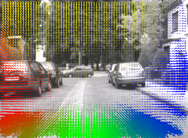
Optical flow calculated from a driving car scene.
Compared with conventional methods for detecting movement, such as calculating the difference between images, CVB Optical Flow not only allows detection but also the quantitative determination of moving image contents, making the algorithm robust against poor or rapidly changing light conditions as well as vibrations. This makes the tool ideal for industrial, traffic and surveillance applications. It supports a variety of monochrome and color formats and it can be used for on-the-fly processing of camera input or to post-process readily captured single images or video data.
Image processing tool for determination of optical flow in images
The evaluation of the optical flow in video images is a key component for automated vision. A reliable detection of local motion vectors is important for a full analysis of complex scenes. However, the general complexity of tracing the former position of an image portion is accompanied by problems like ambiguities, as well as changing lighting conditions and occlusions, which is the reason why there is no simple algorithm available like for other processing tasks. There are different methods known for evaluating the optical flow, each of them having their own advantages and disadvantages. The CVB Optical Flow is based on a variant of the so called block matching approach. In this method, an image and a reference image are subdivided into smaller portions, into so called image blocks. The optical flow is obtained by finding the average shift of the image content within the block-pairs from the two images. Repeating this for many locations of the image will give a high resolution estimation of the motion vectors.
For finding the local shifts efficiently, the CVB Optical Flow utilizes a unique method for performing the cross-correlation for each of the block-pairs extremely fast. Together with the possibility of overlapping blocks and the capability of setting an arbitrary block-size, the common drawbacks of block-matching methods could be eliminated while keeping advantages like flexible spatial resolutions, detection of large motions even for small objects and robustness against many optical disturbances.
One of the goals in the development of the CVB Optical Flow was to keep its usage simple and yet flexible. Once it is initialized, all that needs to be done is to apply the tool to a pair of images or, in case of image sequences, to each of the incoming images. The tool will store the vector components of the local motions separately in simple data-arrays. In addition it will also store a quality indicator for the result at each pixel. Functions for visualizing the results will assist you in evaluating your results.
The CVB Optical Flow functionality can be grouped into three parts. The following sections will describe all steps that are required for determining the optical flow:
Initialization
Calculating the optical flow
Visualization
The first step in using the CVB Optical Flow is to initialize the tool by calling the OptFlowCreate-function. The initialization step is necessary to allocate and to manage memory and to adjust the internal processing functions for the requirements, specific for the sequence. The following information need to be passed over to the initialization-function prior to any other function calls:
This initialization step must be carried out exactly once, before the first tool-function is invoked. The initialization function returns a CVB Optical Flow handle that is required by the processing functions. As long as none of the above mentioned requirements change, there is no need for another initialization, even if unrelated image sequences are being processed. However, e.g. for sequences with different image dimensions, each of them requires its own instance, i.e. its own initialization. Several instances for the CVB Optical Flow may exist at the same time. Due to memory and performance reasons, it is recommended to keep the number of instances as low as possible. After the processing is finished, each handle has to be released again by means of the OptFlowDestroy-function.
To calculate the CVB Optical Flow, the functions OptFlowCalculate or OptFlowCalculateSeq need to be called. After a successful call, they will store the following results in three separate float arrays:
The values in the array will be updated with each function call of the calculation functions. The following parameters are important for calculating the optical flow:
The vector components Vx and Vy, describe the local motion that an image structure has undergone from the reference image to the current image. For these values, the CVB Optical Flow uses the standard computer graphics coordinate system:
Coordinate system used by the CVB Optical Flow.
The following results will be obtained when the image content from the reference image has undergone a motion:
| Motion | left | right | up | down |
|---|---|---|---|---|
| Result | Vx < 0 | Vx > 0 | Vy < 0 | Vy > 0 |
The base of the vector V result will be stored at the pixel position of the reference image.
The block size is a central parameter in the block matching process. The maximum detectable shift of a structure as well as the resolvability of neighbored motion components depend on its size. The maximum detectable x- and y-components of the motion vector V will be half the size of the correlation block. Within a block, the resulting vector represents an average for all motions within. In general, a smaller block size increases the resolvability of neighbored motions, while larger blocks increase the detectable shift range. Since larger blocks also increase the computation time, it is recommended to choose their size just large enough to be able to detect the largest expected motion components.
Motions larger than half the size of the correlation block can also be detected using the rangeExtension-parameter in OptFlowCreate. This will extend the range of the detectable motion components by reducing the resolution of the input images internally by a factor rangeExtension before calculating the flow field. The maximum detection range using range extension will be ±½ blockSize * rangeExtension. In contrast to simply increasing the block size, a reduction of the image resolution will decrease the computation time for a given motion range. If rangeExtension > 1 is chosen, the quality of the evaluated flow results might be affected,because important details in the image might vanish. The magnitudes of the returned motion vectors always represent the motions in the image with original resolution. This means, the magnitude of the resulting vectors does not scale using rangeExtension.
The centers of the blocks are positioned on lattice points of a regular grid, during the calculation process. The tool uses a grid with equal lattice spacing in horizontal and vertical direction. The value for the lattice spacing can be freely chosen during the initialization step and depending on this value, and on the block size, the block boundaries can overlap significantly. With this value, the lateral resolution of the optical flow calculation can be controlled. Choosing an integer value of n for the lattice spacing means that for every n-th pixel a motion vector will be evaluated. For all other pixels, the components Vx,Vy of the motion vector, as well as the correlation value Vc, will be set to zero. The lattice spacing directly influences the processing time, since it controls the number evaluated motion vectors.
Please note: The value n defines the lattice spacing for the internal image. Depending on the parameter rangeExtension, the internal image might have a different resolution than the original image. The distance of the grid points transformed to the original image size is rangeExtension * n.
In order to reduce the computation time, the CVB Optical Flow performs an internal segmentation of the input images. In this step, it is checked whether there are significant changes in the texture between the two images for each image block. In regions where the texture of an image has not changed from one image to another, the optical flow does not need to be computed and the components Vx,Vy of the motion vector as well as the correlation value Vc will be set to zero at this location. Thus, the motion vectors will only be evaluated in areas where a motion with a magnitude larger than zero can be expected. The sensitivity for texture changes is defined by the user.
Choosing a lattice spacing of n, the block matching will be performed for every n-th pixel. A dense flow map, i.e. flow results for each pixel, can be obtained in two ways. The first possibility is to set n = 1 and rangeExtension = 1, which will give the most precise results. However, this will cost a lot of computation time.
In most cases however it is more efficient to choose a value of n > 1 and/or rangeExtension > 1 and to obtain the motion vectors between the lattice points by interpolation. For this, the CVB Optical Flow offers three different interpolation methods, which will automatically create a dense field of motion vectors in the original image resolution from the values at the lattice points. If no interpolation is chosen, only the lattice points will have valid results.
The CVB Optical Flow offers the possibility to create time-averaged results of the flow vectors. This option is controlled by the variable interFrameFilter, which can be set during the initialization step. If a value interFrameFilter > 1 is chosen, then the results for the components Vx,Vy,Vc represent time-averaged values for the respective component. The average is taken across the flow maps of the interFrameFilter frames. The default for this value is set to interFrameFilter = 1, which means that no averaging is performed on the results.
Please note: Using the time-averaging will cause a delayed response of the results to the real motions in the images. Also singular motion-events in time might be possibly removed. Therefore, this option has to be chosen very carefully. It is useful for quasi-static motion fields, i.e. a for constant or a slowly changing motions in images, or for visualization purposes.
In addition to the components of the motion vectors, the OptFlowCalculate or OptFlowCalculateSeq-functions will also return values Vc for each pixel, which indicate how reliable the obtained results are. These floating-point numbers, ranging from 0.0 to 1.0, describe the degree of structural correlation between the two image blocks. A value of 1.0 means that the blocks match perfectly after shifting them back and a value of 0.0 indicates that no structural correlation between these two blocks could be found. As a rule of thumb, if Vc is larger than 0.20, the the components Vx,Vy can be considered to be trustworthy. For lower values the results might still describe the correct motion, but they should be used with caution.
Please Note: It is very important to verify the validity of the result for each pixel before further processing.
The CVB Optical Flow offers two functions for the visualization of the optical flow. These functions can be useful to find the proper parameters for your scenery or the can assist you to evaluate your results. In both visualization functions the direction is coded by using the following color-key chart:
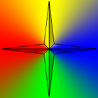
Color key for directions of the vectors.
Please be aware, that the visualization might consume a considerable amount of computation time. In both functions neither the results of optical flow calculation, nor the reference image need to be submitted explicitly to this function. Instead, they are being extracted from the opticalFlow handle. The color overlay image will be written to a compatible CVB image object, which needs to be created by means of the function OptFlowCreateCompatibleImg by the user.
If the reference image was submitted as a color image to OptFlowCalculate or OptFlowCalculateSeq, the pixels will be automatically converted to monochrome values.
For dense optical flow fields the directions of motion vectors can be visualized as a transparent color value overlay on top of a monochrome copy of the reference image.
Please note: In terms of visibility, the function is best suited for dense optical flow fields. These are obtained, if the value for latticeSpacing is not too big or if the results for pixels between lattice points are obtained by interpolation.
In other cases, i.e. choosing interpolation = OFI_None, the visibility of the color overly might not be sufficient if the lattice points are far apart from each other.
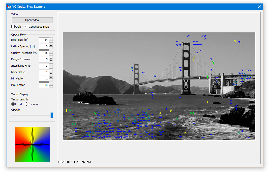
For sparse optical flow fields the motion vectors can be visualized by means of transparent arrows on top of a monochrome copy of the reference image.
Please note: In terms of visibility, the function is best suited for sparse optical flow fields. For using this function, it is recommended to choose interpolation = OFI_None when calculating the flow field.
Examples using the OpticalFlow.dll functions can be found in:
| C# | Common Vision Blox > Tutorial > OpticalFlow > CSharp > CSOpticalFlow |
| VC | Common Vision Blox > Tutorial > OpticalFlow > VC > VCOpticalFlow |
| Delphi | Common Vision Blox > Tutorial > OpticalFlow > Delphi > DelphiOpticalFlow |