|
|
Common Vision Blox 14.0
|
|
|
Common Vision Blox 14.0
|

Common Vision Blox Foundation Package Tool
 C-Style |  C++ | ") .Net API (C#, VB, F#) |  Python |
| CVMetric.dll | Cvb::Foundation::Metric | Stemmer.Cvb.Foundation.Metric | cvb.foundation |
Many image processing applications require calibrations in order to be able to measure features. This applies to both, 2D and 3D applications. The Metric Tool of Common Vision Blox currently provides functionality for the calibration of 3D sensors. In detail, the calibration of laser triangulation systems can be determined (intrinsic calibration). Furthermore, all pre-calibrated 3D sensors can be transformed into a desired world coordinate system (extrinsic calibration).
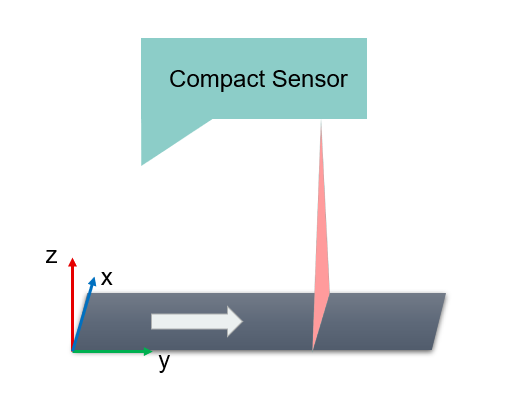
Laser Triangulation
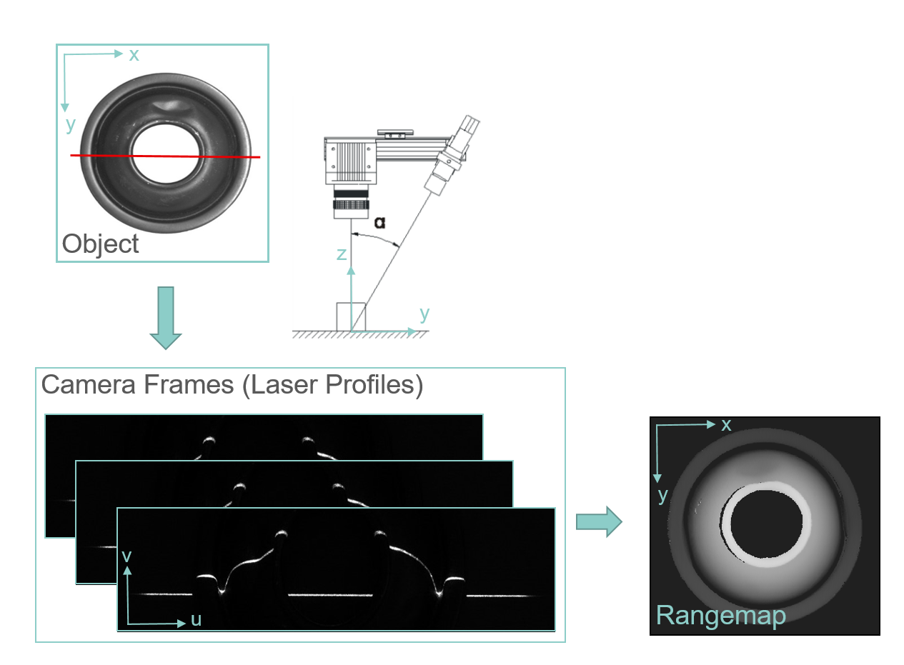
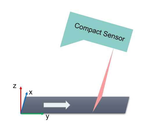
The principle of laser triangulation is shown in the figure below. A line laser emits light to provide a visible line on an object. The profile of the laser line is acquired by a camera that is mounted in a fixed angle to the laser. The shape of the object's surface will define the position where the laser line is captured in the camera sensor. From the distinct pixel positions of the laser line in the image a height profile can be calculated with relative height information. However, without knowing the exact positions and orientations of laser and camera it is not possible to refer these pixel positions to real metric coordinates. Therefore, it is necessary to previously calibrate the triangulation system with a calibration target with known coordinates. By continuously moving the object under the laser-camera-system multiple profiles can be generated and accumulated in one height image. We call those images range maps. The coordinate system of a point cloud created from a range map of a laser triangulation system is defined as follows:
| laser triangulation setup | range map | point cloud |
|---|---|---|
| lateral position on laser line |
number of column in range map image coordinate u of camera frame | x-coordinate |
| position in the direction of movement | number of row in range map | y-coordinate |
| position in the direction of the laser projection |
grey value in range map image coordinate v of camera frame | z-coordinate |
The columns in the range map (x coordinate) correspond to the columns of the raw sensor image (u coordinate). The lines indicate the n'th profile in traverse direction (y direction) and the intensity value represents the v coordinate of the laser peak within the frame.
In order to get 3D world coordinates, the relationship between range map pixels and metric units have to be determined.
Therefore the relationship between pixel coordinates (in the sensor plane of camera) and coordinates of the laser plane, the so-called intrinsic parameters have to be estimated first.
Second, the relationship between laser plane and world coordinates, the so-called extrinsic parameters have to be determined.
The calibration of imaging devices can be divided into two parts: the intrinsic and the extrinsic calibration. The theory behind is described in the section Metric conversion.
The section How to calibrate with CVB explains how to estimate the calibration parameters with Metric using a suitable calibration target.
The metric conversion can be divided into two parts: The intrinsic and the extrinsic calibration.
The figure below gives an overview of the intrinsic and extrinsic calibration parameters. Parameters highlighted in green can be calculated with CVB. The estimation of parameters highlighted in grey is not implemented yet. CVB functions, which calculate the according parameters are marked with a yellow star. The single intrinsic and extrinsic parameters are described in detail in the following sections.


Intrinsic calibration
In order to get highly accurate coordinates lens distortion (e.g. Brown-Conrad, cubic or polynomial) and laser line distortion (2nd, 3rd, or 4th order polynomial) should be estimated. The calculation of these parameters will be implemented in a future CVB release. For 3D compact sensors with built in lasers usually the correction of lens and laser line distortion is provided and can be used before calibrating with CVB.
The relationship between camera pixel coordinates u and v and laser plane (xz plane) is described by the homography H (3x3 homogenous matrix). The homography can be calculated with the CVB function CVMAQS12CreateIntrinsicCalibratorFromPiece. After applying the homography the x and z coordinates of the laser plane are metric. In order to transform the range map rows to metric y coordinates, the velocity of the conveyer belt and the frame rate of the camera (encoder step) must be known.
If the xz coordinates of the laser plane are highly accurate, however the accuracy of the measurement can be reduced by an inclined laser plane. If the laser plane is not exactly vertical to the moving direction (y axis), additional errors are induced. A rotation of the laser plane about the x axis causes shear in yz and scaling in z. In the figure below the acquisition of a cuboid by a 3D laser triangulation system is shown (side view). The errors induced by an inclined laser plane are drawn schematically.

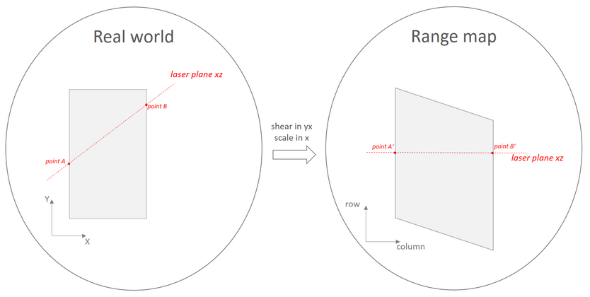
If the laser plane is rotated about the z axis, shear in yx and scaling in x is caused. In the figure below again the acquisition of a cuboid is shown, but from a different view point (view from above). The errors caused by the inclination are drawn in the range map schematically.
These errors can be corrected by an affine transformation. The affine transformation can be calculated by the CVB function CVMAQS12CreateIntrinsicCalibratorFromPiece or - if homography is already known - by CVMAQS12CalculateCorrectionOfLaserPlaneInclinationFromPiece. Note, that the affine transformation also estimates scaling in y, i.e. the encoder step does not have to be known. After the affine transformation all coordinates are metric.
Extrinsic calibration
For the extrinsic calibration a rigid body transformation (rotation matrix and translation vector) is conducted by the CVB function CVMAQS12CalculateRigidBodyTransformationFromPiece. The extrinsic calibration can only be applied if the range map is already calibrated by the intrinsic parameters, which possibly applies for compact sensors, where the distance and the angle between camera and laser line is fixed. In addition the laser plane xz should be just vertical to the moving direction (y axis). If this cannot be guaranteed, it is recommended to use CVMAQS12CalculateCorrectionOfLaserPlaneInclinationFromPiece in order to estimate an affine transformation correcting errors induced by an inclined laser plane.
In order to estimate the intrinsic and extrinsic parameters, a calibration target, where the reference points are precisely known is necessary. CVB currently supports a diamond shaped calibration pattern (AQS12) for both intrinsic and extrinsic calibration. The AQS12 is described in detail in the next section.
AQS12 The AQS12 has a distinct shape with 8 planes and 12 feature points resulting from the intersection points of these planes. The overall size of the target can vary, however, the proportions of the pattern are important for the internal algorithm, as well as the order of the points located on the pattern.

The dimensions of the calibration target should be similar to the example shown in the figures below. In any case it should meet the following requirements:
Note, that the x-axis in the range map represents the x-axis of the camera frame. The y-axis is the traverse direction. The z-axis should be perpendicular to the base plane and represents the height of the object.
In addition the following specifications should be considered during the acquisition:
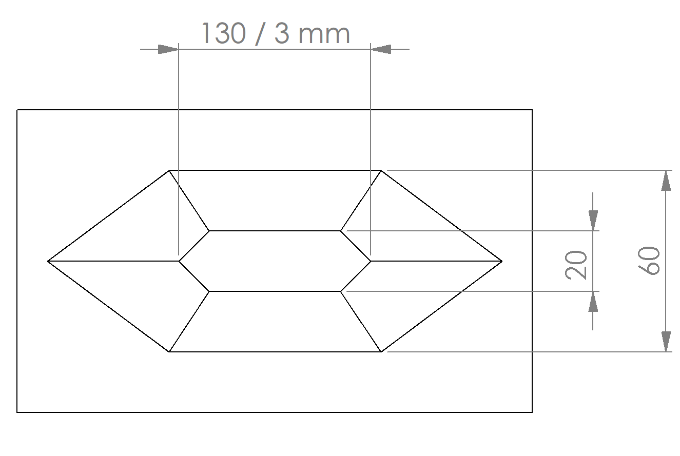
Example dimensions
Top view
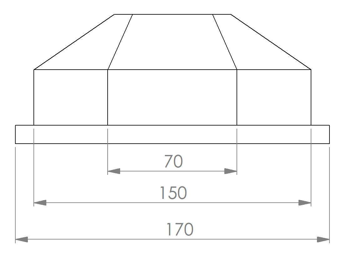
Side view (long side)
Side view (short side)
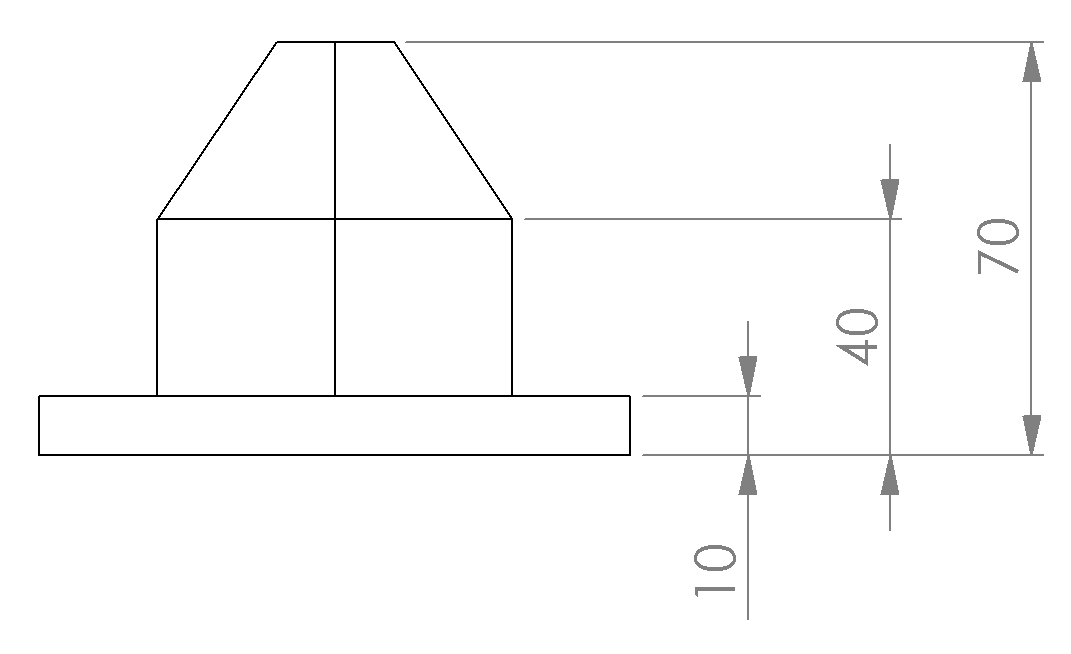
The world coordinates of the reference points for the example shown in the figure above are listed in the table below:
| Point | X [mm] | Y [mm] | Z [mm] | |
|---|---|---|---|---|
| right-handed | left-handed | |||
| 1 | 0 | 110 | 40 | 60 |
| 2 | 10 | 96.667 | 53.333 | 60 |
| 3 | 10 | 53.333 | 96.667 | 60 |
| 4 | 0 | 40 | 110 | 60 |
| 5 | -10 | 53.333 | 96.667 | 60 |
| 6 | -10 | 96.667 | 53.333 | 60 |
| 7 | 0 | 150 | 0 | 30 |
| 8 | 30 | 110 | 40 | 30 |
| 9 | 30 | 40 | 110 | 30 |
| 10 | 0 | 0 | 150 | 30 |
| 11 | -30 | 40 | 110 | 30 |
| 12 | -30 | 110 | 40 | 30 |
| Height | 60 | |||
The first column indicates the x, second the y and third the z coordinate. Mind the order of the points (see Figure above). The single value in the last line represents the height distance between the roof and the base plane. Note, that this value is optional. With this value the height (z value) of the base plane is computed. If it is missing, the height of the base plane is supposed to be zero.
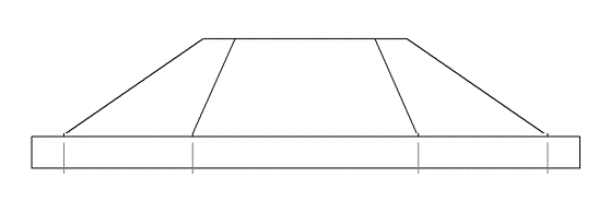
Note, that the vertical walls of the calibration target are not required. The calibration target may also have only the base and the top plane and 6 faces (see figure below).
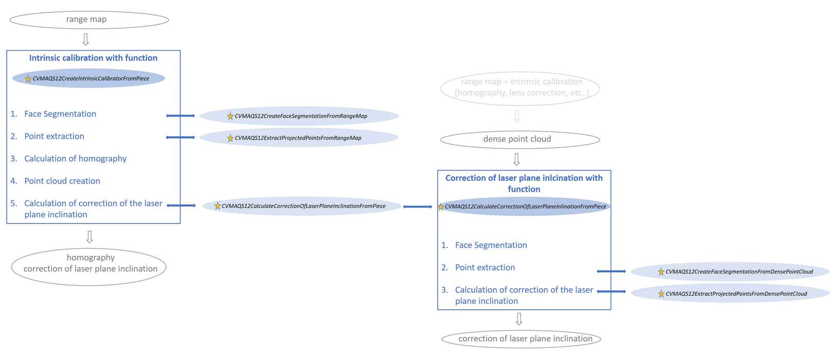
CVB 13.3 provides functions, which return the segmented label image of the AQS12 (CVMAQS12CreateFaceSegmentationImageFromRangeMap, CVMAQS12CreateFaceSegmentationImageFromRangeMapRect, CVMAQS12CreateFaceSegmentationImageFromDensePointCloud, and CVMAQS12CreateFaceSegmentationImageFromDensePointCloudRect) or the extracted points (CVMAQS12ExtractProjectedPointsFromRangeMap, CVMAQS12ExtractProjectedPointsFromRangeMapRect, CVMAQS12ExtractProjectedPointsFromDensePointCloud, and CVMAQS12ExtractProjectedPointsFromDensePointCloudRect). This can be useful, if the user wants to check intermediate results, like the face segmentation or the point extraction.
Note, that the world coordinate system is defined by the given reference coordinates (see table above). By default a calibrated point cloud should be in a right-handed trihedron. But, in some cases, the user likes to do further image processing on a rectified point cloud. Then it is recommended to transform the point cloud to a left-handed trihedron, as the image coordinates are left-handed, too. If he rectifies a right-handed point cloud, the y coordinates will be mirrored in the range map. The figure below shows the calibrated and rectified point clouds in a right- and left-handed trihedron. Please note that in the 3D images in the center column the axis indicators are not located at the actual origin positions for better visibility! The actual origin position - in accordance with the table above - is the point right below corner #7 for the left-handed coordinate system and the point below corner #10 for the right-handed coordinate system.

For the estimation of the calibration parameters with CVB, a suitable calibration target with precisely known dimensions is needed. Until now only the diamond shaped AQS12 is supported (see section above). The CVB calibration functions need as input the accurate coordinates of the feature points (reference) and a range map of the AQS12 (and possibly known intrinsic parameters). First the faces of the AQS12 are segmented on the range map using the kmeans as clustering algorithm. After that a plane is fitted to each face and the intersection point between three neighboring planes is computed. With the intersection points and the precise reference points an affine transformation is estimated. In addition the residuals are returned in each calibration function. The residuals are a good indicator for the accuracy which can be achieved by the calibration. Note that, the residuals relate only to the area of the AQS12. Acquisitions far from the target may be more erroneous, as residual errors propagate with an increasing distance to the calibration target.
The two figures below show the metric functions calculating the intrinsic and extrinsic calibration. In the boxes the internal calculation is described. Several steps can also be calculated separately since CVB release 13.3 (see functions marked with a star). With them, the user can check intermediate results like face segmentation and point extraction in case of an unsuccessful calibration.

In section Calibration Setup typical acquisition scenarios and their solution with CVB are described.
Note, that the calibration functions of release 13.3 and higher expect two object handles which have to be created before. One is needed for the segmentation and one for the intrinsic calibration:
CVMAQS12SEGMENTOR2D for range maps with range map ignore value equal zero. This segmentor has to be used for CVMAQS12CreateIntrinsicCalibratorFromPiece. Function CVMAQS12CreateSegmentorForDensePointCloud creates a default segmentation object CVMAQS12SEGMENTOR3D object for dense point clouds. This segmentor has to be used for CVMAQS12CalculateCorrectionOfLaserPlaneInclinationFromPiece and CVMAQS12CalculateRigidBodyTransformationFromPiece. Note, that background values have to be set as non-confident in the point cloud.CVMAQS12CALCONFIG, where the flags to calculate homography and the correction of the laser plane inclination is set.There are several possibilities to acquire accurate x,y,z coordinates of objects with 3D sensors. The individual calibration workflow you should follow depends on the device chosen and the setup of the camera and the laser. E.g. Area 3D compact sensors already provide a point cloud in metric units. In this case only an extrinsic calibration which moves the points to a world coordinate system is required. Other than with 3D compact sensors with built in laser which usually provide high precision intrinsic calibration parameters (lens and laser line correction and homography). But here in most cases, it cannot be guaranteed, that the laser plane is exactly vertical to the direction of movement. Therefore the estimation of an affine matrix (which corrects errors induced by an inclined laser plane) is necessary. Laser triangulation systems with individual components (camera and laser separated) need both: intrinsic calibration parameters (like homography) and the correction of the laser plane inclination.
The following table shows three typical use cases. They are described in detail below.
| Use Case | Prerequisites | Calibration with CVB and Typical Setup | ||
|---|---|---|---|---|
|
Intrinsic calibration parameters (homography, lens correction,...) | encoder step | Laser plane is exactly vertical aligned to the direction of movement | ||
| 1 | NO | NO | NO | CVMAQS12CreateIntrinsicCalibratorFromPiece -> homography -> affine transformation (rotation, translation, scaling and shear) corrects the laser plane inclination Typical Setup:
|
| 2 | YES | NO | NO | CVMAQS12CalculateCorrectionOfLaserPlaneInclinationFromPiece<p>-> affine transformation (rotation, translation, scaling and shear) corrects the laser plane inclination Typical Setup:
|
| 3 | YES | YES | YES | [CVMCalculateRigidBodyTransformation] CVMAQS12CalculateRigidBodyTransformationFromPiece -> transformation matrix (only rotation and translation) Typical Setup:
|
Use Case 1:

Workflow:
If all calibration parameters are unknown, use CVMAQS12CreateIntrinsicCalibratorFromPiece. This function estimates homography and an affine transformation calculating scale in moving direction and correcting possible errors induced by an inclined laser plane. All coordinates (x, y and z) are metric after the transformation.
Use Case 2:
Workflow:
Applying the intrinsic calibration parameters leads to metric x and z coordinates. In order to correct errors induced by the inclined laser plane, an affine transformation should be calculated using CVMAQS12CalculateCorrectionOfLaserPlaneInclinationFromPiece. With the affine transformation also a scale factor in y is included. All coordinates (x, y and z) are metric after the transformation.
Use Case 3:

Workflow:
Area 3D compact sensors provide point clouds with metric x,y and z coordinates. They usually have to be transformed to a given world coordinate system, which can be done via a rigid body transformation. The target coordinate system is given by the reference points of the AQS12. CVB function CVMAQS12CalculateRigidBodyTransformationFromPiece estimates a rigid body transformation including only rotation and translation.
Use Case 3b: Note, that this workflow is only recommended, if the laser plane is exactly vertical to the direction of movement! If you cannot ensure that, please apply use case 2!
Workflow:
In this case after applying the given calibration parameters the range map values are already transformed to metric x, y and z coordinates. As the laser plane is just vertical to the moving direction, shear in y is not expected. Therefore a simple rigid body transformation can be done with::CVMAQS12CalculateRigidBodyTransformationFromPiece. The rigid body transformation estimates a rotation matrix and translation vector and moves the target to the desired coordinate system given by the reference points of the AQS12.
Sometimes the calibration is not successful or the results are not as accurate as hoped for. There a several reasons for that. The figure below shows the user, what he can do in order to improve his results.
If the calibration ran without an error, he should check the residuals first. If the residuals are smaller than the desired accuracy, the calibration was successful. But attention, the residuals relate only to the area of the AQS12! Acquisitions far from the target may be more erroneous, as residual errors propagate with an increasing distance to the calibration target. Therefore it is very important, that the area where objects will be measured in future is (more or less) completely covered by the calibration piece.
If the residuals are too high, you should check the following:
