|
|
Common Vision Blox 14.0
|
|
|
Common Vision Blox 14.0
|
Common Vision Blox Tool
 C-Style |  C++ | ") .Net API (C#, VB, F#) |  Python |
| CVSpectral.dll | Cvb::Spectral | cvb.spectral |
With the Spectral Dll, CVB introduces a tool to work with hyperspectral imaging data. This library helps and extends CVB and gives the user the ability to work with hyperspectral data while using the experience from the classic image processing market. We introduce image cubes as the container to work with for hyperspectral data. These cubes can be created with any GenICam compliant device. In addition to the pixel values, these cubes contain meta data like wavelengths and FWHM. Fast cube handling is realized by manipulating the view instead of copying the buffer. For cubes in the visible spectrum conversions to XYZ, CIELab and RGB are supported. In addition to our traditional classic C-API, we created object oriented wrappers in C++, .Net and Python.
Features:
To understand Hyperspectral Imaging (HSI) it is important to understand the theory and the techniques behind it. This follwoing sections contain the most important topics covered by the library. They start off with: How does the acquisition of hyperspectral imaging data work? After acquiring these data, how do you model this data in your software? To save these cubes to memory and share with other people and programs we use the widely supported file format ENVI-format. There is also a short introduction on color conversion to XYZ and Lab.
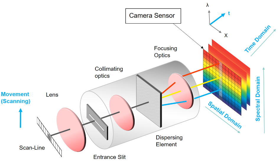
All cameras capture scenes of the world. But the resulting image may vary depending on the camera sensor. For instance a camera with a monochrome sensor will integrate all wavelengths in its sensitivity curve. This results in an image with one plane. In contrast a Bayer-sensor (typically used by RGB cameras) has a specific filter for each channel. The resulting image has three planes. A hyper spectral camera will create an image with n planes. However, how do you acquire these images or cubes? The most popular approach for acquiring a high number of bands is the Pushbroom Spectrograph.
The Pushbroom approach uses a dispersion element to split an incoming beam into different beams. The exit angle of the resulting beam is dependent on the wavelength. Theses beams will hit a sensor with an appropriate spectral sensitivity. In the image below the y-axis of the sensor is used to differentiate between different wavelengths. The x-axis is used to achieve a spatial resolution. While this approach may yield a high number of bands the resulting image will only contain one spatial axis. Therefore this camera can be seen as a line scan camera. The acquired image only contains one spatial axis. A relative movement between camera and object will create a whole scan of the object. This scanning movement will therefore create the remaining spatial axis.
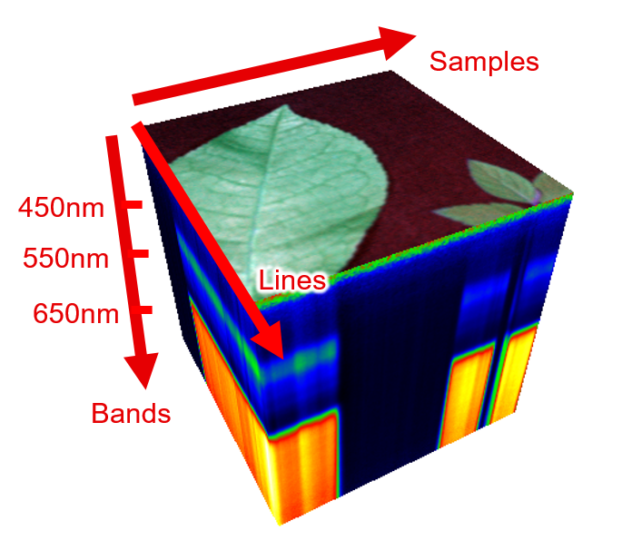
All cubes contain an n-planed image (IImageVPA) and metadata (SpectralMetaData). The image is the result of a scan with a hyper spectral camera, when each image is placed in a separate plane of an image. The metadata is needed to assign each dimension of the image to either a spectral (bands), spatial (samples) or a temporal (lines) dimension. Furthermore it contains the wavelength for each band.
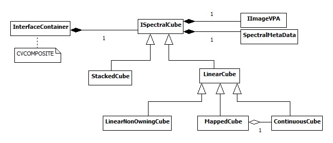
The UML-diagram above visualizes the different kind of cubes offered by the C-API. Each of these cube types have their own use-case:
All pixel values are stored in a continuous buffer with a fixed increment. Therefore linear cube owns the continuous buffer. This cube supports all mapping operations without the need to copy any buffer.
Mapped cubes are created by applying an operation on a continuous cube without copying any buffer. This allows fast operations like cropping or transposing. All pixel access operations are therefore passed onto the original continuous cube. Consequently changing pixel values of a mapped cube will also change the ones in the continuous cube. To ensure that this memory is not deleted the mapped cube holds a shared pointer of the continuous cube. The metadata however is independent from its continuous cube.
This cube type allows the creation of a cube from any given buffer without copying this buffer. The only restriction is that the pixel access is linear: x-, y- and z-increments are therefor constant.
Can be created from an array of single planed images without copying any buffer. The typical use-case is when creating a cube from the ring buffer. There is no restriction on the location of each image in memory. Therefore there is no constant z-increment and the cube is not linear. Some fast mapping operations may not work on this cube. To enable these, it is necessary to create a continuous cube from a stacked cube first.
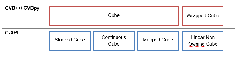
The CVB++ and CVBpy interface wraps the C-API of CVB. In contrast to the four different types offered by the C-API the CVBpy interface offers only two distinct kinds of Cube classes: Cube and Wrapped Cube The Cube class is used for Continuous Cube, Mapped Cube and Stacked Cube. Wrapped Cube is a subclass of Cube. It covers the use case for Linear Non-Owning Cubes. Consequently, an instance of this class does not own its image buffer. You could create a Wrapped Cube by simply passing the base pointer as well as the increments for samples, lines and bands.
Each Cube contains a way to access an n-planed image and the describing spectral Meta Data. The Meta Data describes the image in a spectral manner. The image itself does not contain any information about which of the axis is assigned to the spectral axis. Interleaved Type contains this information.
| BandInterleavedByLine | [x, y, z] → [samples, bands, lines] |
| BandSequential | [x, y, z] → [samples, lines, bands] |
| BandInterleavedByPixel | [x, y, z] → [bands, samples, lines] |
Wavelengths contains a float vector used for the wavelength-to-band mapping. This field is optional.
All available fields can be accessed by the following functions. FieldID is an enum class with all supported fields. Please note that these template functions are only defined for the following data types:
There are two possibilities to access each pixel of the cube. Either by using the underlying image (BufferView) or by using the LinearAccess method in the Spectral library. The biggest difference between them is the dimensions to iterate over.
Also known as duplicate. Continuous cubes offer the biggest flexibility for mapped operations, which do not require any copying of the buffer eg. transpose and crop. To create a continuous cube out of any given type of cube use the clone method.
Transposing a cube means to change the view on the buffer. The buffer view has the dimensions x,y,z while the cube contains the dimensions samples, lines, bands. A transpose operation changes this dimensional mapping.
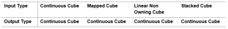
In the C-API there are two distinct function to either create a Mapped Cube or to create a Continuous Cube. In the object oriented wrappers (CVB++ and CVBpy) there is only one function. When this function is called it tries to create a Mapped Cube. The advantage is that such an operation is very fast as no memory is copied. This is however only possible if the original cube contains a linear buffer. This is true for all cubes except for Stacked Cubes. In this case, Transpose creates a Continuous Cube. The table further below visualizes this relationship. To force the new Cube to be completely independent from the original data use the Clone function afterwards. Otherwise, any change on the original buffer will be visible in the resulting cube. The following table visualizes which Cube Type are created when using this operation in the object oriented case (CVB++ and CVBpy):
![]()
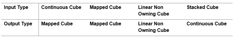
Also known as map. This operation creates a Cube out of a given sub space. Using this operation it is possible to create a cube, which only contains the area of interest spacial and spectral wise. In the C-API there are two distinct function to either create a Mapped Cube or to create a Continuous Cube. In the object oriented wrappers (CVB++ and CVBpy) there is only one function. This function tries to create a Mapped Cube as this avoids copying any buffer. This is only possible for Continuous and Mapped Cubes as input. For Stacked Cubes Map outputs a Continuous Cube. To force the new Cube to be completely independent from the original data use the Clone functionality afterwards. Otherwise, any change on the original buffer will be visible in the resulting cube. The following table visualizes which Cube Type are created when using this operation in the object oriented case (CVB++ and CVBpy):
The following table shows the resulting Cube Type for each combination of input cube type (first row) and operation (first column):
| Operation \ Input cube Type | Continuous Cube | Linear Non-Owning Cube | Mapped Cube | Stacked Cube |
|---|---|---|---|---|
| Clone | Continuous Cube | Continuous Cube | Continuous Cube | Continuous Cube |
| Transpose (mapped) | Mapped Cube | LinearNonOwningCube | Mapped Cube | N/A |
| Transpose (buffer) | Continuous Cube | Continuous Cube | Continuous Cube | Continuous Cube |
| Slice | IMG | IMG | IMG | IMG |
| Crop (mapped) | Mapped Cube | LinearNonOwningCube | Mapped Cube | Stacked Cube |
| Crop (buffer) | Continuous Cube | Continuous Cube | Continuous Cube | Continuous Cube |
| +-*/ | Continuous Cube | Continuous Cube | Continuous Cube | Continuous Cube |
| Normalize | Continuous Cube | Continuous Cube | Continuous Cube | N/A |
The ENVI-format is an open file format commonly used to store hyperspectral imaging data. The format consists of two files, a header file and a buffer file.
This ASCII file ('.hdr') works as the descriptor for the buffer file. It contains the information on how to interpret the buffer file. This Meta Data is structured in fields, each having an ID, a name and a value. The ID is used to access a field. The name is a string as defined in the ENVI-format. The following list contains a number of notable fields:
| BandInterleavedByLine | [x, y, z] → [samples, bands, lines] |
| BandSequential | [x, y, z] → [samples, lines, bands] |
| BandInterleavedByPixel | [x, y, z] → [bands, samples, lines] |
This file contains the image as binary data with the extension '.bin'. The information on how to parse this data is given in the header file.
The spectrum of cubes in the visible range can be converted to a color metric. This library covers XYZ, CIE Lab and sRGB. As for pre-processing, a normalization is essential to be remove the spectral dependency to the whole setup.
The spectral density as acquired by a hyperspectral device contains the combination of spectral responses from illumination, environment, optics, spectroscope, sensor and of course sample. To extract the reflectance spectral density of the sample it is necessary to normalize such an image cube. This is done using a white and a black reference. Effectively this gives a relative response with respect to the given white reference. Therefore, it is important to have a white reference with an uniform reflectance spectrum. The resulting values of the image cube are in the range [0,1].
Currently the only available normalization method is NormalizationMethod::AverageReferences1

Effectively this gives a relative response with respect to the given white reference. Therefore, it is important to have a white reference with a uniform reflectance spectrum. The resulting values of the image cube are in the range [0,1]. The three cubes S, BRef and WRef need to have the same dimensions for Bands. In the Lines and Bands dimension the Reference Cubes are averaged to estimate the expected reference.
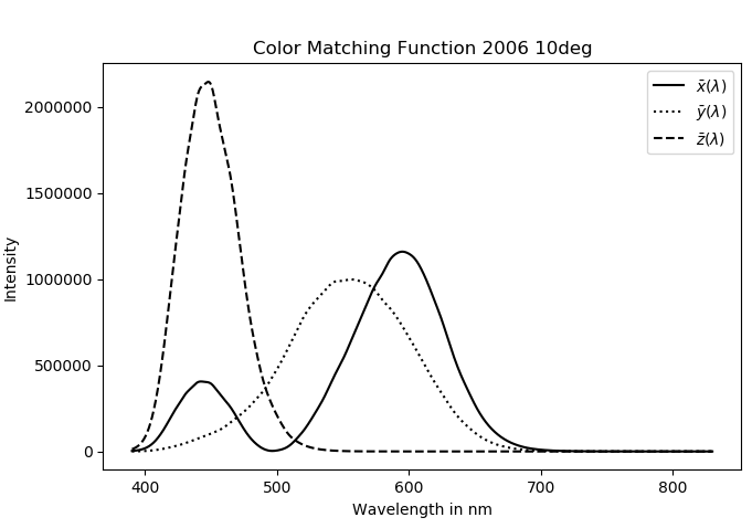
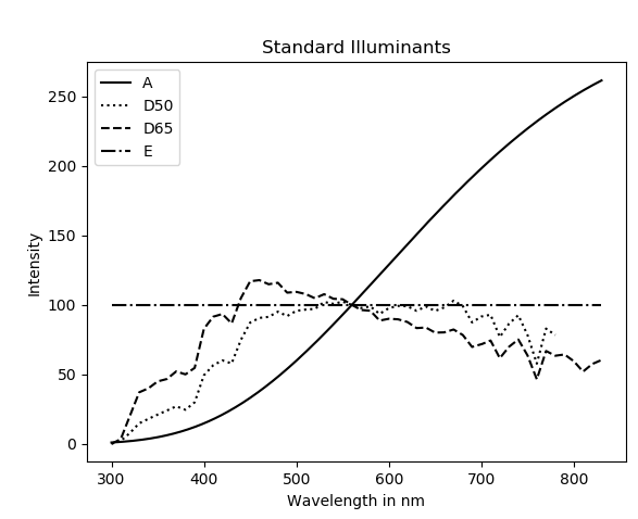
The tristimululs or XYZ color space is often the starting point for many other color spaces. In this color space the spectral sensitivity of the human eye is applied. The calculations are done using the color matching functions. These functions are curves, which describe the spectral sensitivity of the photoreceptors in the human eye. The CIE standard defines a number of Standard Observer to address this matter. Reflective or transmissive objects by itself do not emit any light. To calculate the XYZ- tristimulus value for these objects an additional Standard Illumination is needed. For this purpose the CIE standard defines a number of Standard Illuminats.
To calculate the XYZ-tristimulus values the following formula is then applied:
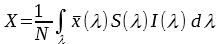
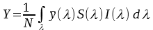
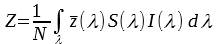
with
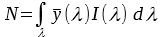


Prior to applying this calculation the wavelength grid of the normalized sample S(λ), the Color Matching Functions and the Standard Illuminant need to be aligned. Therefore, an Interpolator is created. It access the meta data Wavelength of the given cube and uses this wavelength grid as the target for color matching functions and Standard Illuminant. This Interpolator then contains the spectral densities of the standard illuminant and the color matching functions in the same grid as the normalized sample cube S(λ). This Interpolator is then used to calculate the XYZ image.
The most popular metric to express color is the CIE Lab Color Space defined by the CIE (Commission internationale de l'éclairage). CIE Lab holds the three values L, a and b in the value range [0, 100] [-128, 127] [-128, 127] and is relative to a given white point. This color space is device independent and therefore can be used to compare different colors.
To convert from XYZ-tristimulus to CIE Lab (L*,a*,b*) a reference white point is needed . Typically, the white point of the standard illuminant D50 or D65 is used.

with


Similar to the calculation of the Trisimulus XYZ this calculation requires an Interpolator with the correct wavelength grid. The Lab image can be calculated using the Cube or by using the XYZ image
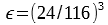
Neither XYZ nor CIE Lab values can be shown on screen properly. For this purpose sRGB is used. Currently the conversion is only defined for sRGB with D65 as standard illuminant.
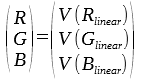
with

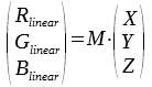
with 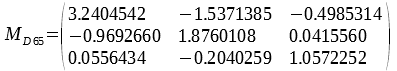
The Interpolator is used for the internal intermediate conversion from Lab to XYZ.
Examples using the CVSpectral.dll functions can be found in:
| C++ | Common Vision Blox > Tutorial > Spectral > Cvb++ > CubeAcquisition |
| C++ | Common Vision Blox > Tutorial > Spectral > Cvb++ > ColorConvert |
| CvbPy | Common Vision Blox > Tutorial > Spectral > CvbPy > ColorConvert |