|
|
Common Vision Blox 14.0
|
|
|
Common Vision Blox 14.0
|

Common Vision Blox Tool
 C-Style |  C++ | ") .Net API (C#, VB, F#) |  Python |
| Polimago.dll | Cvb::Polimago | Stemmer.Cvb.Polimago | cvb.polimago |
Polimago is a software package to aid the development of applications in machine vision for:
in a broad range of possible environments, encompassing industrial or medical imaging, human face detection or the classification of organic objects. The underlying technological paradigm machine learning and training is an essential part of application development using Polimago. The package contains applications for:
The library functions are described in the API-part of this documentation. They also include functions needed for training, thus users can create their own training programs.
Before doing so, users are advised to familiarize themselves with the supplied programs to acquire a thorough understanding of the training procedures. The following section "Classification and Function Estimation" tries to answer a question of the type "what is it?" concerning a fixed image and a range of possible answers, corresponding to potentially very different objects. "Image Search" tries to answer the question "where is it?" concerning a fixed object type and a range of answers, corresponding to different locations and possibly also very different states of rotation and scaling.
Although Classification and Function Estimation on the one hand and Image Search on the other hand are based on the same machine learning technology and are often intertwined in applications, they are somewhat different problems requiring different training procedures.
Here, we give a brief overview.
Polimago generally operates on images provided by the Common Vision Blox Image Manager. The input images, however, must meet certain criteria for Polimago to work on them:
MapTo8Bit() (CVCImg.dll), ConvertTo8BPPUnsigned() or ScaleTo8BPPUnsigned() (CVFoundation.dll) as they provide the functionality required to correct the bit depth.CreateImageSubList() (CVCImg.dll) may be applied to reduce the number of planes.GetLinearAccess().GetLinearAccess() returns FALSE you may use e.g. CreateDuplicateImageEx() (CVCImg.dll) to correct the image's data layout.GetLinearAccess() function by looking at the increments returned for the individual planes. CreateDuplicateImageEx() may be used to correct the memory layout.Condition 3 and 4 are usually only violated if the source image has been pre-processed e.g. with CreateImageMap() (CVCImg.dll) or if the images have been acquired using some very old equipment. Otherwise these conditions are usually met 99% of the time.
The theory of operation includes a tutorial which serves as the practical part of this documentation. In seven lessons all relevant aspects of Polimago are presented - from the testing and training of search classifiers to different classification tasks.
Classification and function estimation (or regression) are concerned with the analysis of a given image rectangle of given size, as defined by a fixed position in some image and a fixed reference frame. There are two forms of application:
In both cases training is based on a sample database consisting of labeled examples.
A sample database is a set of pairs (I,L) where
The information contained in the sample is then processed by the machine learning algorithm to create a classifier, a data structure which can be used to analyze future image rectangles. The user can contribute to the quality of the classifier in three ways:
Image search is concerned with the analysis of entire, possibly very large, images. The image is searched for occurrences of a pattern or objects of a single type. For each occurrence information about the geometric state (position, rotation, scale, etc) is returned.
While classification and regression are implemented in Polimago following standard machine learning techniques, image search combines these methods in a more complex process, somewhat resembling the saccadic motion of human eyes.
The basic idea is the following: looking at an image rectangle defined by a current position and a current reference frame (which can include parameters like rotation and scaling), we are faced with three possibilities:
Such a search procedure can be reduced to a number of tasks involving classification and regression, and can be trained using the corresponding methods.
The entire training process becomes a lot more complicated. In Polimago it is encapsulated in dedicated training functions creating a search classifier - a data structure which parametrizes the entire search procedure and contains many elementary classifiers and function estimators. Polimago comes with a dedicated training application for search classifiers, accompanied by a training tutorial.
Users who wish to use the search-functionality of Polimago are recommended to go through all the steps of the tutorial before embarking in their first project.
The frame is called the Feature Window. Features inside the Feature Window are relevant for the definition of the pattern.
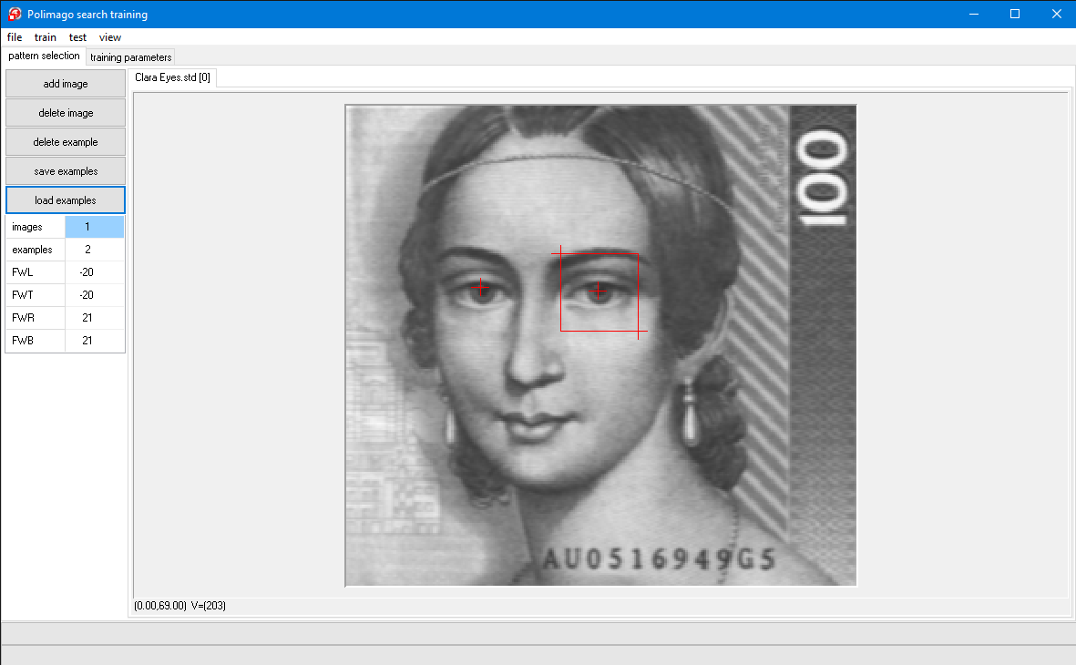
The extension .psc stands for "polimago search classifier" and the file you have opened is a search classifier, which we have already trained to find Clara Schumann's eyes. The file name is shown in the program window's caption line.
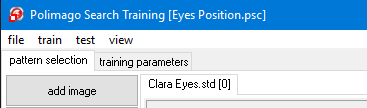
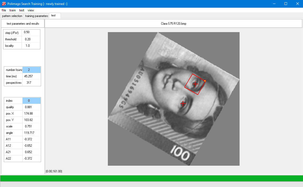
An image of Clara Schumann appears. The tab "test" is activated. We will test the search classifier on this image. Since we wish to start with something easy, we chose the same image which was used for training.
You have activated the API-function PMGridSearch() using the current classifier SearchClf() as a parameter. The image is searched and the results are displayed.
The left-hand side of the program window shows three parameter fields with parameter names and associated values. The top field contains some parameters of PMGridSearch() which will be explained later. The other two parameter fields are output parameters of this function. The middle parameter field shows:
The image itself shows two cross-hair overlays at the two eyes, one at each returned solution. One solution is highlighted by a frame drawn around it which has the same size as the feature window. The properties of this selected solution are shown in the bottom parameter field on the left. Important are the:
The quality can be larger than 1, this will be explained in later lessons. You will notice that also the coordinates have fractional values.
Polimago-search always returns sub pixel coordinates.
The other parameters in the bottom parameter field will be explained later. They are irrelevant at the moment. Using test/next or F7 you can switch between the two solutions, with corresponding parameters shown on the left. Alternatively you can just left-click on the cross-hairs.
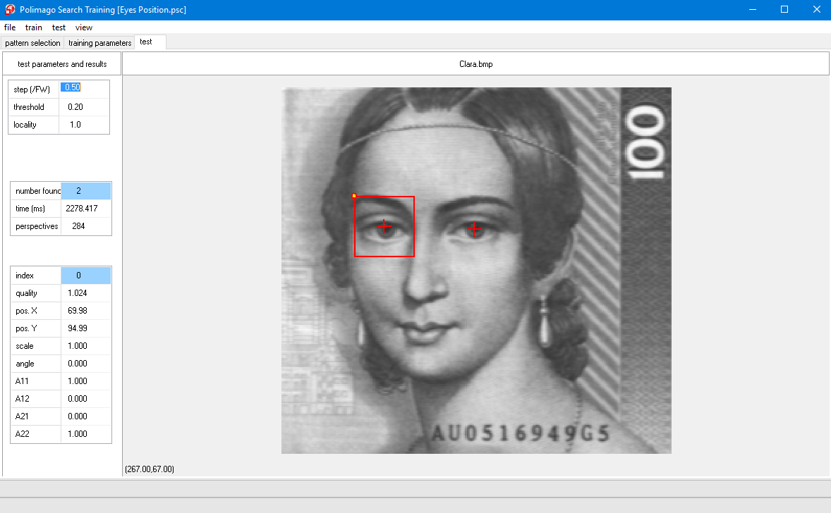
If you select view/perspective (which is then checked) you will also see the content of the highlighted frame on the right-hand side of the program window (refer screenshot next chapter).
We now come to the control parameters in the top left parameter field. These are:
Step(/FW):
This is the step size of the grid used by PMGridSearch() in units of the size of the feature window (more precisely the unit is the minimum of height and width of the feature window). It corresponds to the API parameter Step.
So if the feature window is 40x40, as in the given case, and the step is 0.5, then a parameter field of 20x20 pixels is searched. This means that an elementary search process PMInspect() is started at every twentieth pixel in every twentieth line in the image. A coarse grid, corresponding to a larger step size, is faster, but it may fail to catch the pattern.
Please experiment with this by selecting test/search (F8) for different values of the step parameter (say from 0.1 to 1.5), observing execution time and success of the search each time, then set it back to default=0.5.
Threshold:
This is a quality threshold for returned solutions. Set it to 1 to find that now only the left eye is found (or none for >1 ), then set it back to default=0.2.
Locality:
This controls how close solutions are allowed to be located to each other. It is again expressed in feature-window units. Try the value 4 to find that it now finds only one of the two eyes, then set it back to the default value 1.
We conclude this lesson with some additional feature exercises:
Default area is the entire image. To return to it click the LEFT button somewhere in the image.
Continue from the last lesson, or, if you have shut down the program in the meantime:
Use file/open test image (F3) and file/open sc (F4) to load the image "Clara.bmp" and the search classifier "Eyes Position.sc" located in %CVB%Tutorial/Polimago/Images/QuickTeach, respectively.
When you drop the "start"-label a feature window frame appears centered at the label together with some other cross-hairs in the image.
The image on the right-hand side shows the contents of the frame centered at "start" and the caption "initial perspective". This is the starting point of an elementary search process with PMInspect(). If done right, you will see a part of an eye somewhere in the image on the right-hand side below "initial perspective" (otherwise drag "start" again to correct).
At this point the input data of the elementary search process are the pixel values of the image on the right-hand side, just as you see it. We call the corresponding frame in the big image window the Perspective. Since the perspective contains part of an eye, there is enough information to shift it to the eye's center (approximated).
This is intuitively obvious to you by just looking at the image on the right-hand side. The search classifier "Eyes Position.sc" contains a function, or rule, which computes a corresponding transformation from this image, which is just a two-dimensional vector used to shift the perspective.
You will notice that the transformation has been carried out and the new perspective has centered the eye to a first approximation, which is probably already quite accurate.
The caption is now "perspective at stage 1". The content of this perspective is the input for the second stage of the elementary search process.
In principle one could now use the displacement function as before for another approximation. But, since the obtained approximation is already much better than the initial state, the input is more regular and smaller displacements have to be predicted. Therefore a new, more accurate, function is being used at the next stage.
If you use next (F7) two more times and you were close enough to the eye initially, you will arrive at the center of the eye and the image on the right will be labeled "final perspective, success".
The elementary search process mimics the way in which you modify your own perspective to get a better view of some interesting object - through eye movements, by turning your head, or changing the position of your body.
As you step through the stages of the elementary search (using test/next of F7) you can monitor the respective quality and position values on the bottom parameter field on the left-hand side.
You may wonder why the final quality is often lower than the previous one, even though the final approximation appears at least as good. This is because the final quality is computed as a running average of the previous ones. Thus making the quality measure more stable and to favor elementary search processes with initial position already close to the target.
Now drag the start-label far away from the eyes and step through the approximation procedure. Typically you will encounter a failure ("final perspective, failure") already after the first approximation step.
To get a feeling for the elementary search process, please play with many different start-positions, near and far from the eyes. You will come to the following conclusions:
The API-function PMGridSearch() initiates an elementary search process at every grid-point as specified by the area of interest Left, Top, Right, Bottom and the spacing parameter Step, and retains every successful solution with quality above the parameter Threshold in a list of Results. This list is pruned by retaining only solutions of maximal quality within a given diameter: the Locality. The number of perspectives processed is returned as NumCalls.
A far reaching conclusion is reached if you move start to one of the good initial positions. For instance, you could chose the initial position in a way, that the image on the right-hand side contains a good portion of one of the eyes. Even if the eye in the initial perspective has been rotated or scaled you would know how to compensate this by rotating, scaling and shifting your own perspective to approximately center the eye in its normal state of rotation and scaling. This observation can be seen as the basis of invariant pattern searches, a topic we explore in the next lesson.
With the tab pattern selection opened,
You should drag the cross-hairs around and resize the feature window, delete cross-hairs or add new ones by clicking in the image.
The zoom-function of the right mouse-button may be helpful.
After playing around with these possibilities please load "Clara Eyes.std" again so that we can continue from a defined state.
At the bottom of the column labeled "current training parameters" there is a combo-box, which, in the default-state, is set to "affine".
Here you can define the type of invariants which you want to train. You will see that there are three possibilities defined by the InvarianceType:
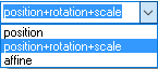
Select "position+rotation+scale" and then "train/train" from the menu. You have initiated the training process two progress bars will start moving at the bottom of the program window. If you look at the "current training parameters" you find that the parameter NumClfs is set to 6, the default setting of the program. That means that elementary search is at most a 6-stage process.
At each stage we need two functions:
This means that now we have to train 12 classifiers. Correspondingly, the upper of the two progress bars moves in twelve segments that move until the training is finished. You can train again (train/train, don't save the classifier) to observe this process.
A search will find the two eyes again. Now look at the values on the bottom parameter field on the left-hand side of the program window.
You will find that the scale and angle are measured to reasonable accuracy. These values are not quite equal for the two eyes. This is not surprising, because they are also slightly different patterns.
In the parameter field below scale and angle are the four entries of the corresponding transformation matrix. The individual parameters of a search result are recovered by the API-functions PMGetXY(), PMGetScaleAngle() and PMGetMatrix() respectively. The Quality is a field of the structure TSearchResult.
Now play with the trace function at different positions near and far from the pattern. Also try the image "Clara S120 R300.bmp", which has been scaled by 120% and rotated by 300° (=-60°). Also try the image "C5799.bmp" which has undergone an additional shearing transformation and really requires affine invariants. Nevertheless, the current classifier should be able to locate the two eyes and determine approximate scale and orientation with somewhat distorted final perspectives.
affine, re-train (“train/train”), and experiment with the resulting search classifier.The correct result is now given by the coefficients A11, A12, A21 and A22 of the transformation matrix. Scale and angle are now only approximations.
By now you will have realized that one of the key ingredients of an elementary search process are the functions which effect the changes in perspective. From a perspective content, these functions compute the transformations which modify position, scale, angle, and even the shape of the current perspective frame.
The transformations are described by vectors which are two-, four-, or six-dimensional for the training modes of "position", "position+rotation+scale" and "affine" respectively. Correspondingly the transformation functions to be learned for each stage have two, four or six values.
In this lesson you will learn how these functions are being trained. Please go to the tab training parameters and examine the column labeled current training parameters. You see two groups of parameters:
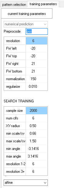
The topmost parameter in this group is called "sample size", also called SampleSize in the API. This is, for each training step, the number of examples considered for processing. The default value 2000 is a good starting point for most applications. For difficult problems with four- or six- dimensional invariants you may require a larger value. This considerably slows down the training time (3rd power of sample size), but does not directly affect the execution time of a search.
The parameter "numclfs" (NumClfs in the API) determines the number of elementary search stages to be passed until success and has been explained in Lesson 3. The transformation functions are trained from examples and the next 5 parameters directly affect the generation of these examples.
To obtain these examples random perspectives are generated as randomly transformed feature windows about the position of the training pattern.
We then have to find a function which, from the contents of such a random perspective, computes the right transformation to find back to the right perspective, which is just the original feature window about the position of the training pattern. But this right transformation is just the inverse of the transformation with which the random perspective was generated. So the pair (perspective content, inverse transformation) is a randomly generated (input, output)-example of the function to be found.
The total number of such examples is given by SampleSize. The algorithm then determines a function which approximates the corresponding inverse transformation for each example. The method of regularized least squares is used. The coefficients parameterizing this function are stored with the classifier.
This function has as many components as the corresponding transformations. We first consider the most simple case of the "position" invariance, where there are only two components for the shift in X- and Y-direction respectively.
The question one could ask would be: Which random transformations can be used? For higher stages of the elementary search we need only smaller transformations (in the sense that they effect smaller changes). But, even for the initial stage it makes no sense to generate perspectives which do not overlap with the original feature window because they could contain no more information about the original pattern and its position.
A good rule of thumb are shifts by at most 0.5 times the minimum of the feature window's width and height for the first stage. This is the default value of the parameter XYRadius. So if, for example, the feature window is 20x20 with the pattern position at the center, the examples are generated by shifting the window randomly by up to 10 pixels in each direction. If such a shifting transformation is given by (dX, dY) then (-dX, -dY) is the inverse which has to be learned.
The space of possible transformations (or perspective changes) is a square of side length 21, from which the training examples are chosen. So, the algorithm attempts to locate the pattern from a distance of roughly XY-radius times the size of the feature window. This means that the Step in the search parameters can be chosen accordingly.
The situation is a bit more complicated for the case of "position+rotation+scale" invariance. In addition to the simple shift there are now two more parameters governing orientation and scale of a perspective in a way, that the training examples have to be chosen from a four-dimensional volume. The simple shifts are again controlled by the parameter XYRadius.
In addition to this the scale is delimited by the parameters MinScaleMinL and MaxScaleMaxL, while rotation is delimited by MinAngle and MaxAngle. The scale parameters are in natural units (multiplied by 100 to obtain %), the rotation parameters are expressed in radian.
If you want to train a classifier which is rotation-, but not scale-invariant, set both MinScaleMinL and MaxScaleMaxL to 1.0. The example volume is then only three dimensional, the density of examples is higher and you will obtain more accurate results as with additional scale invariance. Similarly, if the classifier shall be scale-, but not rotation-invariant, set MinAngle and MaxAngle to zero.
The default setting yield full rotation invariance and scale-invariance from 2/3 to 3/2 of the pattern size, a range of 9/4 which lies a little over the factor 2. Clearly, there are limits to scale invariance: a pattern may loose relevant features when down-scaled too much and acquire irrelevant features when up-scaled too much. Don't expect anything reasonable outside the range from 0.5 to 2.
The situation is similar for the "affine" invariance, only the example volume is now 6-dimensional. The delimiting parameters now refer to the singular value decomposition (short SVD) of the generated matrices. The SVD decomposes the matrix into a product of a rotation, a diagonal matrix, and another rotation.
MinScaleMinL and MaxScaleMaxL now give the minimal value for the smaller - and the maximal value for the larger of the singular values. The angular parameters delimit the total rotation implied by the two rotation matrices.
We have described the training of the displacement functions of the initial elementary search stage.
For the subsequent stages random perspectives are generated in exactly the same way, but they have already been corrected by the previous stages, in a way that the example perspectives are closer to target and the corresponding displacements are smaller. At this point you should try to create classifiers which are purely rotation or purely scale invariant.
For instance this could be done for different facial features of Clara Schumann and with different invariance constraints. Using "test/transform image" you can transform the current test image for your experiments.
The other key ingredient of the elementary search process are the functions which decide if the current perspective content has any chance leading to the desired pattern.
These functions are very important for the search performance, because abandoning a search process early can save a lot of execution time. Just like the displacement functions the verification functions are trained from examples.
The number of examples is also controlled by the parameter SampleSize and the examples fall into two classes: promising perspectives and unpromising perspectives.
The algorithm gathers random promising and unpromising perspectives, maintaining a balance between the two sets until the total SampleSize has been reached.
Again, with regularized least squares the verification function is determined which approximately reaches the value 1 (the supposed minimum) at all the promising and the value -1 (the supposed minimum) at all the unpromising perspectives.
This function is not of a binary type, instead, it is continuous so that it can be used for a ranking and rating of perspectives in the training process, and as a quality measure in the search process. The continuity of this function is the reason why returned qualities can be larger than 1.
If you get false negatives, you may have forgotten to mark some positive examples in the training images. It is important to mark all present positives examples.
You will probably notice that PMGridsearch() now finds the right eye as well as other eye-like features, but with lower quality than the left eye. This is because these features are somewhat similar to the left eye and are not included in the training data, thus they are not used as counter-examples. The right eye being correctly recognized is an instance of "generalization" - the recognition of patterns not previously seen in the training data.
Normally you need much more than a single positive example to achieve good generalization, but the two eyes are really similar in this case, thus it yields the result shown. The effect of generalization may be unwanted in case of the other features which are now recognized. To exclude these false positives, add the image "100.bmp" to the training data (you don't need to do anything else with it) and train again.
You will find that the false positives have disappeared, because "100.bmp" contains the false positives which are now used as counter-examples automatically.
The "feature map" is the function which takes an image and a perspective frame as inputs and computes a "feature vector" from it. This feature map is a sequence of numbers describing the image in some way. The feature vector serves as an input for learning and execution of classifiers and numerical estimators.
It is the input for both the transformation and verification functions used in the elementary search processes. The feature map is conceptually a three stage process:
You will not need to compute these granularity, nor will you need to fix the dimensions of the retina - Polimago does it for you. But, you can control the size of the retina through the parameter resolution (range 1 to 10).
In the simplest case of a square feature window the width and height of the retina are given by resolution times granularity. So if the pre-processing code is 'pss' and the resolution is 6, then the retina has width and height of 6*8=48. It is important to realize that this is the case regardless of the size of the feature window.
If the feature window is not square then the two factors which multiply the granularity to obtain width and height of the retina are chosen so that:
This sometimes implies a distortion of the image in the retina.
Sometimes you will see this in "view/perspective" if you work with non-square feature windows, because the image displayed there is really the image of the retina. Making the retina smaller will increase execution speed but can lead to a loss in recognition quality and precision.
In the initial stages of the elementary search the speed is more important. In the final stages precision is more important. That is why we let you choose different resolution parameters for the initial two stages (resolution 1-2) and for the remaining stages (resolution 3+).
Lessons learned from the last two exercises: If you depart too far from the default parameters you may run into unexpected problems.
The pre-processing code is a string which can consist of four different characters.
With the exception of '+' they correspond to processing operations and are executed from left to right.
With "Clara Eyes.std" from %CVB%Tutorial/Polimago/Images/QuickTeach and default parameters try the pre-processing codes 'ps' and 'p' to see that they successively lead to a deterioration of results.
With "view/perspective" you can witness the effect of the pre-processing codes on the size of the retina: 'ps' has granularity 4, so the retinas width and height become 6*4=24, 'p' has granularity 2, so the retinas width and height become 12.
In this final lesson you will be guided through the development of a more sophisticated search classifier.
With the exception of the experiment in Lesson 5 we have only dealt with the recognition of patterns which arose from geometrical transformations of the training pattern. This is hardly realistic in practical situations where there are all kinds of noise, starting from cameras, illumination, dirty objects, or natural deformations of organic objects.
Some of this variability can be covered by examples, but clearly not all. It is therefore necessary that the search classifier generalizes pattern properties from the known examples to unseen situations.
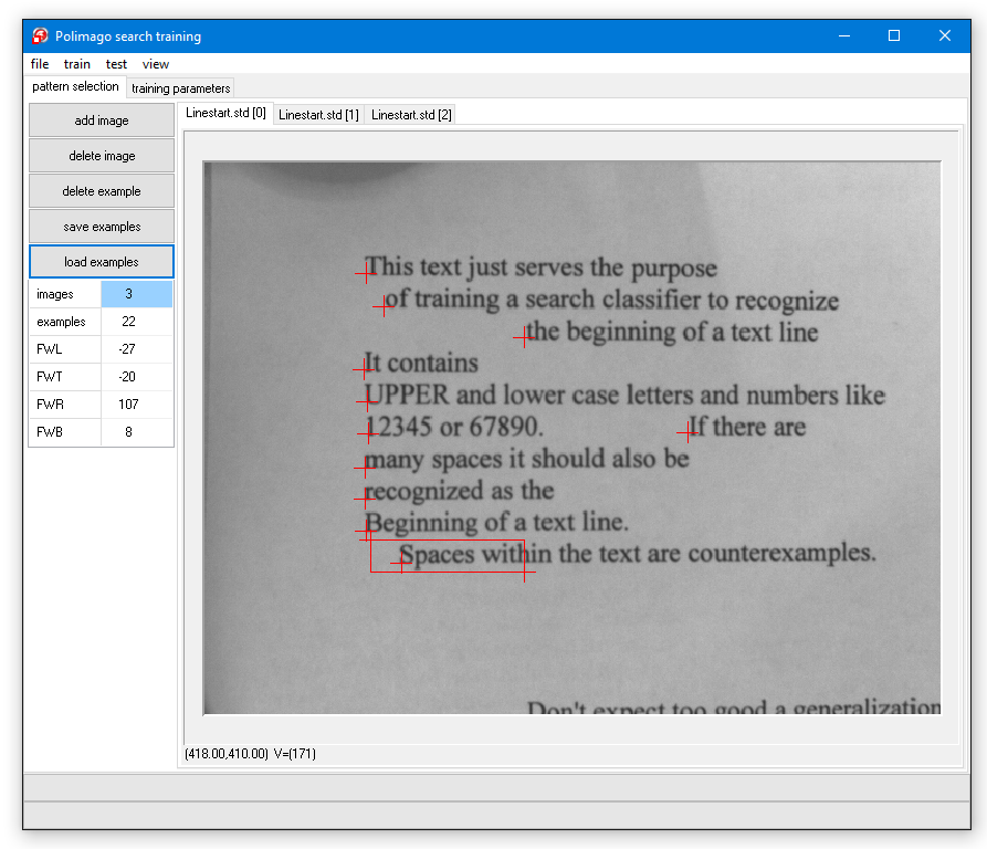
In this lesson we will create a search classifier to locate the beginning of text lines and record their orientation.
This may not be practically useful, as there are probably better methods dedicated to this problem, but it is a well suited use case to acquire some working knowledge of Polimago.
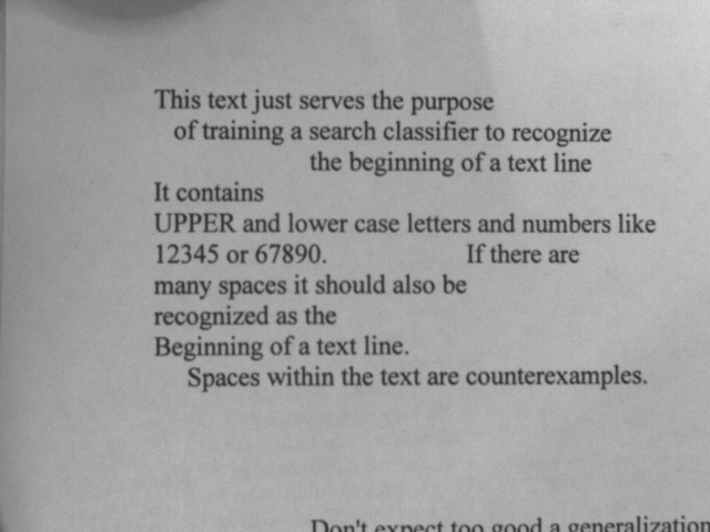
The challenge here is that every line of text may start with another word or numeral and may also be of different font and size.
It is clearly impossible to foresee all possibilities and to provide corresponding examples. To make things a little more difficult we will not only consider horizontal lines, but allow them to be rotated up to plus or minus 45°. We will also tolerate some variation in scale from 70% to 120% of the scale of the training data. invariances

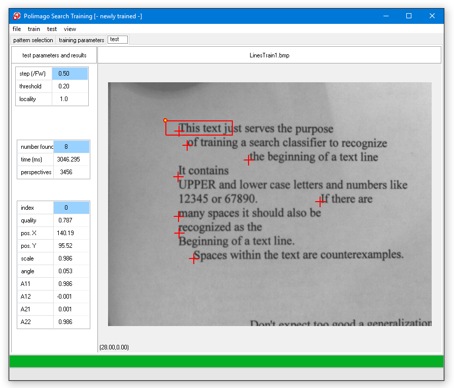
If you try the result after test/search on the loaded test images (file/open test image) "LineTest1.bmp" through "LineTest3.bmp" (it is best to step through the solutions with "view/perspective" switched on), you will find that some lines are not found at all, and that many results are falsely positioned between the lines. This is because the height of the feature window is approximately the distance between two lines in the training set.
With XYRadius equal to 0.5 training perspectives are generated which lie halfway between the lines. These perspectives are highly ambiguous, because it is unclear if they should be shifted to the line above, or to the one below. You will appreciate this ambiguity if you try the trace in "LineTest1.bmp" and position the "start" label between line beginnings.
Another problem is that the ambiguous positions in the training set are too close to the positive examples to serve as counter-examples. The remedy for both problems is to decrease the XYRadius.
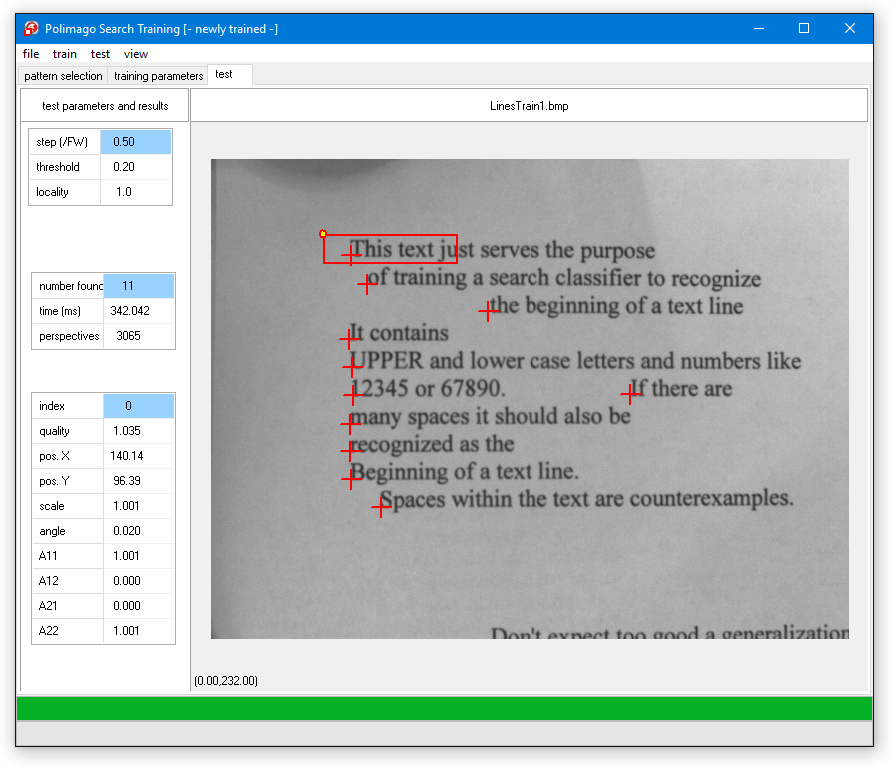
You will find that the previous systematic error has been corrected, but that there is a significant number of false positives - in particular for the more difficult images with fonts and orientation different to the training images. The returned angles and scales are also very imprecise. The reason for this is that the retina is too small.0.
The initial anti-aliasing 'p' in the pre-processing code obscures this fact.

The code 'aa' is about as good as 'pss'.
If you now tested and look at the perspective images, you will find that the perspective is very poorly resolved. In fact, the retina is only 12 pixels tall!

Please train again and test. You will find that the result is a great improvement, although there are still a few false positives.
What else can be optimized? We are training with a sample size of 2000. This means that, on average, each of the rather heterogeneous examples gives rise to about 90 randomly shifted, rotated, and scaled perspectives. This seems to be not much.
When you come back and test the result, you will probably find that there is an improvement, but perhaps the difference is not significant enough to justify the extra training time.
To obtain any real further improvement one would need to enlarge the training set. It is simply not enough to have some examples. More likely you would want 100 examples, perhaps also example images dedicated to exclude false positives. If this is done properly it will help a lot more than the artificial increase in sample size.
Here are a few general hints:
We hope you had a good time experimenting with the search functions of Polimago, and wish you good luck and success with your applications.