|
|
Common Vision Blox 14.0
|
|
|
Common Vision Blox 14.0
|

Common Vision Blox Foundation Package (Windows only!)
 C-Style |  C++ | ") .Net API (C#, VB, F#) |  Python |
| CVCFoundation.dll | Cvb::Foundation | Stemmer.Cvb.Foundation | cvb.foundation |
The Common Vision Blox Foundation Package is a complete easy to use comprehensive collection of optimised image processing functions.
Based on the CVB Image Manager that offers unique functionality in image acquisition, image handling and image processing, it contains an extensive set of image processing functionality allowing you to control many different types of image acquisition hardware, as well as providing an optimised image display.
Basic functionality such as abstract image access is possible using predefined tools as well as user specific algorithms.
It is also easily possible to create special algorithms for your specific application based on the samples delivered for all supported compilers.
In addition to core machine vision technologies the CVB Foundation Package contains an extensive set of optimised algorithms for
It even contains an extensive range of
Beside the Foundation Tools, CVB Foundation offers binaries, header files and tutorials under:
> Common Vision Blox > Tutorial > Foundation (CVBTutorial/Foundation)
Note, that for some tools, ActiveX Controls are available, too:
The separately available components that are bundled in the Common Vision Blox Foundation Package are
(1) Note that the functions of CVB Arithmetic have been superseded by new functions introduced in the Common Vision Blox Foundation Package. Nevertheless, Arithmetic is part of the Package to facilitate an easier migration for existing customers for Arithmetic. However we strongly recommend new customers to use the new arithmetic functions in the Foundation Package.
(2) There is a separate theory of operations chapter available for this topic.
Additional functionality that comes with the Common Vision Blox Foundation Package may roughly be split into the following groups:
(1) The Blob implementation in the Common Vision Blox Foundation Package does not supersede the CVB Blob tool. It is more of a complement to the CVB Blob tool, in that it implements the standard functionality like measurement of center, area and 2nd order moments, but it lacks the ability to measure perimeters, holes or convex projections. It is to a high degree code compatible with CVB Blob, allowing you easy migration to that tool if you should need to make use of the more advanced features of CVB Blob.
For a list of the executables that form the Common Vision Blox Foundation Package, please see CVBTutorial/Foundation.
The bundled tools mentioned in the overview come with all their binaries, header files and tutorials.
Common Vision Blox Foundation Package contains resources for:
CVFoundation DLL
with functions for
Examples can be found in Common Vision Blox Tutorial ˃ Foundation directory.
To use any of the functions in the Foundation Package Libraries it is necessary to include libraries and header files to the development project. These libraries and headers are different for each supported development language.
Find here an example description for a programming approach:
CSharp:
| Libraries | CVFoundation.dll |
|---|---|
| .Net Wrapper Dlls | ../Lib/Net/ iCVFoundation.dll |
| .Net Code documentation | ./Lib/Net/ iCVFoundation.xml |
| Examples | ../Tutorial/Foundation/VB.Net, CSharp,.... |
C++ ( Visual C, VC.Net unmanaged)
| Libraries | CVFoundation.dll and ../Lib/C/CVFoundation.lib |
|---|---|
| Function declarations: | ./Lib/C/ iCVFoundation.h |
| Examples | ../Tutorial/Foundation/VC |

Image Processing Tool for Arithmetic and Logical Operations
There are arithmetic and logical operators as a part of the Common Vision Blox Foundation Package available.
| Examples | |
|---|---|
| VC | Common Vision Blox > Tutorial > Foundation > VC > VCArithmeticSingleImg |
Common Vision Blox > Tutorial > Foundation > VC > VCArithmeticDualImg |

Image Processing Tool for FBlob analysis
FBlob is a part of the Common Vision Blox Foundation Package for measuring various morphometric parameters in objects of any shape (contiguous pixel ranges) which are defined by means of a binary threshold (blobs).
In this process, FBlob does not analyze individual pixels but operates with a representation of contiguous object ranges in an image row – the run length code.
Each image row is coded in such a way that the start address and length in the X direction are stored for every contiguous object range.
This approach speeds up operations considerably compared with a pixel-based or recursion-based algorithm.
Then the adjacency of the object coordinates in the current row to the existing objects is analyzed, and the measurement parameters of these objects are updated accordingly.
Objects can be of any shape and complexity.
It is possible to make the return of measured values dependent on whether an object satisfies certain criteria (filters).
For instance, a size threshold can be set below so that small objects that are frequently generated by noise are not measured, or objects that touch an image border can be suppressed.
The FBlob implementation bears a lot of similarity to the CVB Blob tool that has been available in the Common Vision Blox tool series for many years now.
However the FBlob implementation - compared to CVB Blob - is limited in its capabilities.
While CVB Blob returns a large number of results for the individual blobs, FBlob is limited to the following set of Blob parameters:
If you need more information about your objects we recommend that you use the CVB Blob tool.
The usage and function signatures of FBlob and CVC Blob are built in such a way that those two implementations are almost interchangeable (with the exception of those features that are not common to both implementations).
| Examples | |
|---|---|
| CSharp | CSharp FBlob Example (needs .NET Runtime): Common Vision Blox > Tutorial > Foundation > CSharp > CSFBlobExample |
| VC | VC FBlob Example: Common Vision Blox > Tutorial > Foundation > VC > VCFBlobDemo |

The CVB Foundation package provides a set of functions for colour space conversion.
It supports conversions between the following color modes:
RGB, YUV, YCbCr, XYZ, LUV, Lab, YCC, HLS, HSV
It supports also the conversion from any of the color modes to gray scale and to a custom model by using the following color twist matrix, too.

Related Topics
| Examples | |
|---|---|
| CSharp | Common Vision Blox > Tutorial > Foundation > CSharp > CSColorSpaceConversion |
| VC | Common Vision Blox > Tutorial > Foundation > VC > VCColourSpaceConv |
Description
Color spaces are mathematical models that help us describe colors (e.g. in an image) through a tuple of n numbers (in most color spaces n = 3, sometimes n = 4).
Any color space or color model defines color relative to a certain reference color space.
For example the chromaticity diagrams of the CIE (Commission Internationale de l'Éclairage) that have been designed to encompass all the colors that may be distinguished by the human eye may serve as such a reference (note that these chromaticity diagrams evolved over the years, so it is always necessary to specify to which of the diagrams you actually refer):

In such a chromaticity chart, the principal components of a color space represent a distinct location, and the colors that may be described by a given color model are represented by an area spanned by these principal component points.
One of the most common color models, and certainly one with which any one working with computer is to some degree familiar, is the RGB color model, where a color is derived through the additive mixing of the three principial components red, green and blue.
In PAL broadcast and video compression, the color space YUV or YCbCr is commonly used. Many more models exist, and a subset of them has become accessible in Common Vision Blox through the Color Space Conversion functions found in the CVFoundation.
A more detailed description of the supported color spaces may be found in the discriptions of the respective transformation functions
Recommended Reading:
Color Spaces in CVB
With the inclusion of a set of Color Space conversion functions in the Common Vision Blox Foundation Package, it has become necessary to add to an image object the information about which color space has been used to describe the colors in the image.
Therefore the CVCImg.dll exports the function ImageColorModel, which returns an enumerated value describing the color space that is being used.
Unfortunately, only few acquisition systems and image formats actually give this kind of information.
Therefore a way had to be found, how to treat images that do not have a color space information attached to them, and the following simple heuristic has been chosen:
ImageColorModel (have a look at the Image Dll header file to get the list of possible return values).CM_Guess_Mono (-1) is returned.CM_Guess_RGB (-2) is returned.CM_Unknown (0) is returned.Note that the guessed values have been chosen such that abs( CM_Guess_Mono ) = CM_Mono and abs( CM_Guess_RGB ) = CM_RGB.
Whenever an image is passed to one of the color space conversion functions exported by the CVFoundation.dll, it first checks for the appropriate input format. CM_Guess_RGB is always believed to be an appropriate input format.
For example an image passed to ConvertYUVToRGB must either have the color model CM_YUV (produced by ConvertRGBToYUV) or CM_Guess_RGB (if loaded from a file or from a frame grabber) - otherwise the image will be rejected and the return code 27 (CVC_E_INVALIDCOLORMODEL) will be given to indicate the mistake.

CVFoundation.dll provides functions for image correlation.
Foundation Correlation functions in CVFoundation.dll provides correlation functions such as:
| Examples | |
|---|---|
| VC | Common Vision Blox > Tutorial > Foundation > VC > VCCorrelation |
![]()
CVFoundation.dll provides functions for Foundation Fast Fourier Transform Functions
| Examples | |
|---|---|
| CSharp | Common Vision Blox > Tutorial > Foundation > CSharp > CSFoundationFFT |
| VC | Common Vision Blox > Tutorial > Foundation > VC > VCFFTFilter |
| VC | Common Vision Blox > Tutorial > Foundation > VC > VCFFTScaling |

Image Processing functions for Curves
A curve is a function that maps from a 1D space into a higher dimensional space. For CVB this space is restricted to 2D. Curves are often drawn in 2D and can be confused with graphs that map from 1D to 1D but are also drawn in 2D. These graphs however, map from 1D to 1D. Drawing a circle on an image can be described as a curve, but no graph exists that can do the same. Curves are used to restrict areas or describe general shapes. Curves can be rotated, translated and more while keeping properties of a curve. As such they are an elementary tool in image processing and for describing shapes. 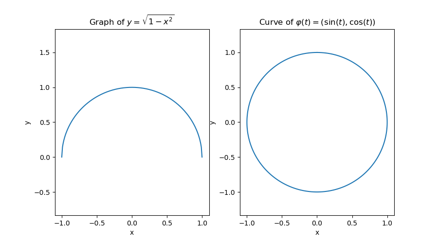
Curves in CVB are represented by a list of ordered points with linear interpolation between them. This is also called a "discrete representation". An example of a spiral curve is depicted in the figure below. On the left side the points are stored in the correct order and the curve is as expected. On the right side the points where shuffled randomly and stored as a list again. When interpreting this shuffled point set as a curve the curve would look like the right image. 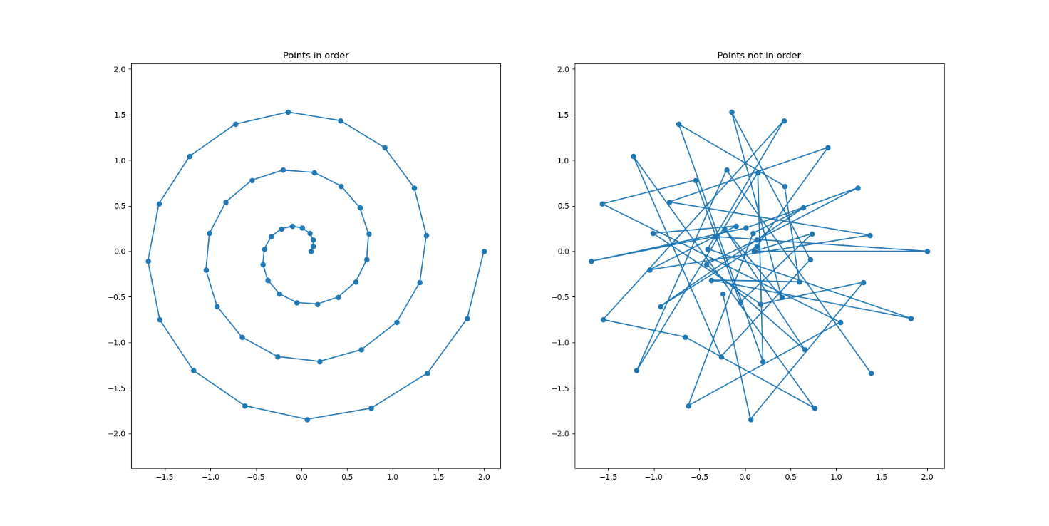
For handling point clouds CVB includes functions to
These functions and their underlying theory is explained in the corresponding subsections.
Some general advice when working with curves:
s(t) = s(2*t).In this section different distances and how they are defined as well as calculated are presented. 
There are three different distances that need to be clarified when considering the distance of a point from a curve. For the remainder of this text the curve is denoted with s(t) and assumed to be represented by an ordered point set. The distance is being calculated with respect to point p (denoted "sample point" in the picture above).
All three different distances are depicted above. A more detailed information about the different distances is given in the text below.
The first distance is a direct result of the way how curves are represented in CVB, which is as a list if points. It is natural to use this representation to directly calculate distances between points and curves. This, however does not account for the linear interpolation between the points in the curve and thus is only an approximation.
A more accurate distance does not only consider the point to point distance between curve s(t) and point p, but interpolates the curve correctly to find the normal distance to the curve. To calculate this distance, first the closest point in the point set representing the curve is found. We denote this point as q1. Then, the neighbor of q1 which is closest to p is selected . We denote this point with q2. The final distance is then calculated between the line going though the selected points, q1 and q2, and the point p.
Since a curve is ordered and there is a direction of traversal from start to end an additional information is available and may be desired: On which side of the curve s(t) the point p is situated. When calculating the point to curve distance with interpolation a hessian normal form is used for calculating the desired distance. This distance is always positive but during the calculation the necessary information about left and right is present. When calculating the distance with side information we denote point on the left with a positive distance and point on the right with a negative distance. Technically speaking, the result is not a distance any more since it doesn't fulfill the mathematical properties of a distance. Using the absolute value of the "signed" distance will resolve this issue. The "signed" distance now includes on which side of the curve the point p is, denoted by its sign, and its distance to the curve.
Intersections
After this thorough examination of distances between points and curves the next topic is how to find intersections between lines and curves. Finding the intersection between a curve and a line can be done by calculating the signed "distance" of each point representing the curve to the given line. The curve and line intersect at a point with distance zero or between two consecutive points with changing sign. Since linear interpolation is applied between two consecutive points in a curve, the exact intersection point can be calculated mathematically by intersecting the two lines.
In CVB all possible intersections are found and stored in a list.
To speed up computation times it can be beneficial to only work with the point set representing a curve. Depending on the distances between points this approximation can be accurate enough while giving a significant performance increase. In some instances points are not distributed uniformly along the curve, this can result from the acquisition or if the curve is generated artificially from a CAD file or mathematical formula. In this case re-sampling the curve to have equidistant points can be helpful. Another reason for re-sampling may be to reduce the overall number of points that need to be stored and processed.
To resample a given curve into n equidistant points, first the overall length of the curve is calculated and divided into n-1 equal parts. Then the curve is re-sampled at the beginning and the calculated length. This ensures that the new points represent the given curve while at the same time being uniformly distributed. An example of a curve with 50 points and its re-sampled counterpart, again with 50 points is shown below. 
While this approach is fast and yields good results it does have two major downsides. Firstly, the new curve was generated from equidistant points but since now the re-sampled curve has different distances between adjacent points due to the linear interpolation, it may not be equally distributed in itself. The figure below illustrates the changes within a curve after resampling (note that the given example will be equidistant after resampling). This effect could be minimized by iterating inversely how the points should be distributed in the original curve. Since in practice the difference should be small, the faster approach was chosen for CVB. 
Secondly, this method does not use any type of smoothing kernel or functional approximation. It will suppress high frequency changes within the curve if the new number of points is lower than the original number of points (see example below), but does not provide any further parameters for fine tuning.
For the denoising example a curve is generated from 500 points equally spaced between 0 and 2π in x and y = sin(x)+δ. The noise δ is generated from a normal distribution with center 0 and scale .08. The resulting curve is re-sampled with 250 points and 50 points. The resulting curves are shown below 
To see the effect on the high frequency noise the three violin plots for each curve and its difference to an ideal sinus curve are shown. 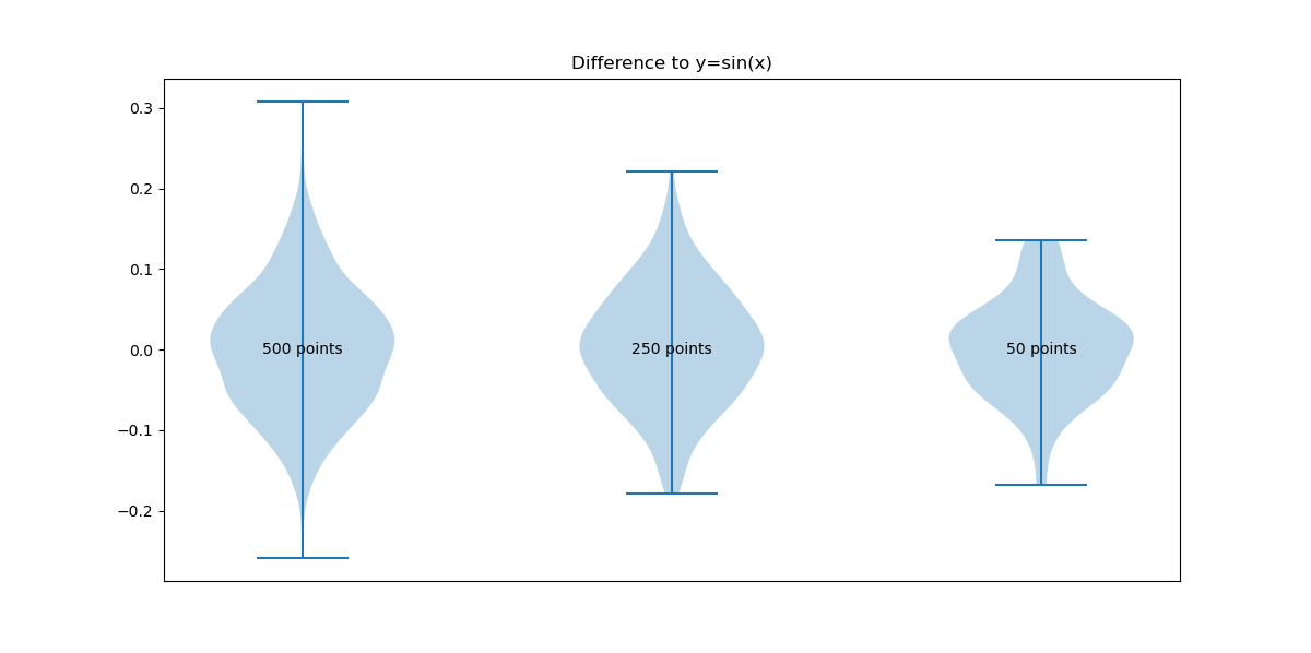
To align two curves an enhanced ICP (iterative closest point) method is implemented. This method allows for fast alignment for curves that may only partly overlap. The input curves are aligned using only the points in the lists without any interpolation. This will ensure that "holes" in the data are not improperly closed which would lead to false information being processed. A typical use case is aligning data from two sensors while the object is only partly visible and/or partly occluded for each sensor. In this case, the data will only represent curves with "holes".
The implemented method is an iterative method which consists of the following steps
More details about the steps and all possible input parameters are listed below. And an example alignment is shown in the following image. 
Finding corresponding pairs and calculate the matching score
Let P1 be the point set representing the first curve and point set P2 represent the second curve. For each point w in P2 the closest neighbor in P1 is found. The found neighbor to w in P1 is denoted v. If the euclidean distance is less than a given threshold, the point pair is considered corresponding to each other. If the value is greater, the closest neighbor of v in P2 is found. This neighbor is denoted w2. If 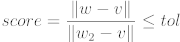
the point pair v, w is considered corresponding to each other.
The set C is the set of found corresponding point pairs. The matching score between the two sets is only calculated over the set of corresponding point pars. Let the set P3 be the subset of P2 that includes all the points that have a corresponding neighbor in P1. The matching sore is then calculated via 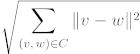
And if no stopping criteria is met, the rigid body transformation between the pairs in C is calculated in a way that minimizes the current matching error. In each iteration of the algorithm the corresponding pairs and thus C is recalculated following the method described above.
Matching score tolerance
If the matching score falls below this threshold, the matching is considered successful and will stop. The default value is 1e-6.
Early stopping criteria
If the matching score does not improve by at least the given tolerance, and early stopping criterion is triggered and the found solution is returned. The default value for this tolerance is 1e-5.
Shape sensitivity
The shape sensitivity is defined by a float value between 0 and 1. A higher value means higher sensitivity. A value of 0 corresponds to the classical ICP without any shape sensitivity. A value between .8-.9 is recommended as default value when aligning curves. This value is not very sensitive, meaning a value of .88 yields similar results to when using .9 as shape sensitivity. This value helps find stable parameters without the need to re-parametrize the function constantly.
Maximum number of iterations
The implemented algorithm is based on the classical ICP algorithm and thus iteratively minimizes the matching discrepancy. The maximum number of iterations restricts the iterations that the algorithm can perform. In most applications the algorithm converges within 30 iterations and thus 40 maximum iterations should be sufficient. The larger the maximum iterations the larger the computation time differences between successful and failed alignments become. If consistency is desired, a small test set should be used for finding a good limit for when convergence should be reached and the maximum number of iterations subsequently be set accordingly.
Restrictions of the method
ICP based methods are local optimizations. As such the alignment depends on the starting positions and rotations of the curves. Local optimization methods have the advantage of being fast and precise but do fail to find a global optimum if the minimization function is non-convex. By introducing shape sensitivity to the classical ICP the provided algorithm is able to converge faster and is less dependent on the starting position and rotation. If multiple matches are possible, this method finds only one, depending on the starting position. See below figure for an example. 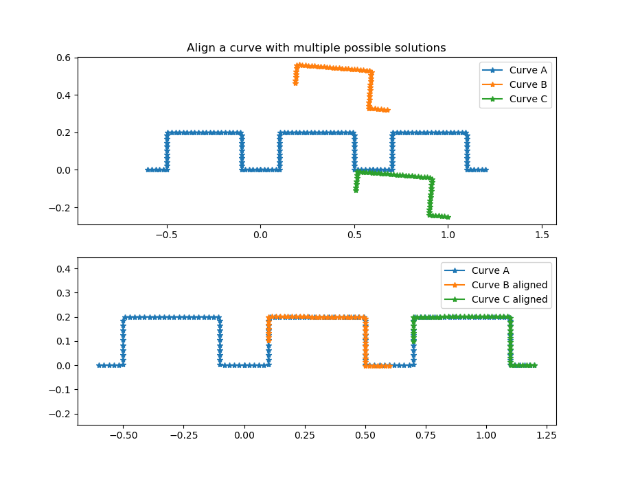
To merge two curves that may overlap we need to have a starting- and end-point for each curve. Just combining the two point lists into one long list will not work if the curves overlap. In this case an average at the overlap or suitable interleaving has to be found. See the image below as an example for a failed merged using the naive approach. 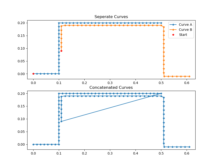
Instead, given two curves for merging, the outcome is supposed to be a single curve that keeps the order in each point set as given while combining both sets with a shortest path. This will ensure that overlapping areas are merged even if they don't match perfectly. To find this shortest path, the implemented algorithm uses nearest neighbor information for each curve and adds interpolation when altering between the two given curves. It is capable of handling curves with holes, and multiple overlaps. 
For a successful merge it is important that the order of the given curves is matching, the matching assumes that the first point in each curve has to be merged before the second point. Detecting the best order (front to back or back to front) is not part of the implemented algorithm. If the two curves were generated from different cameras or sensors, the caller has to make sure that left to right is the same for each camera, or save the curves accordingly before calling the merge function. Below is an example of a merge of two operation where the order was incorrect. A successful merge is shown in the example above on the same data. 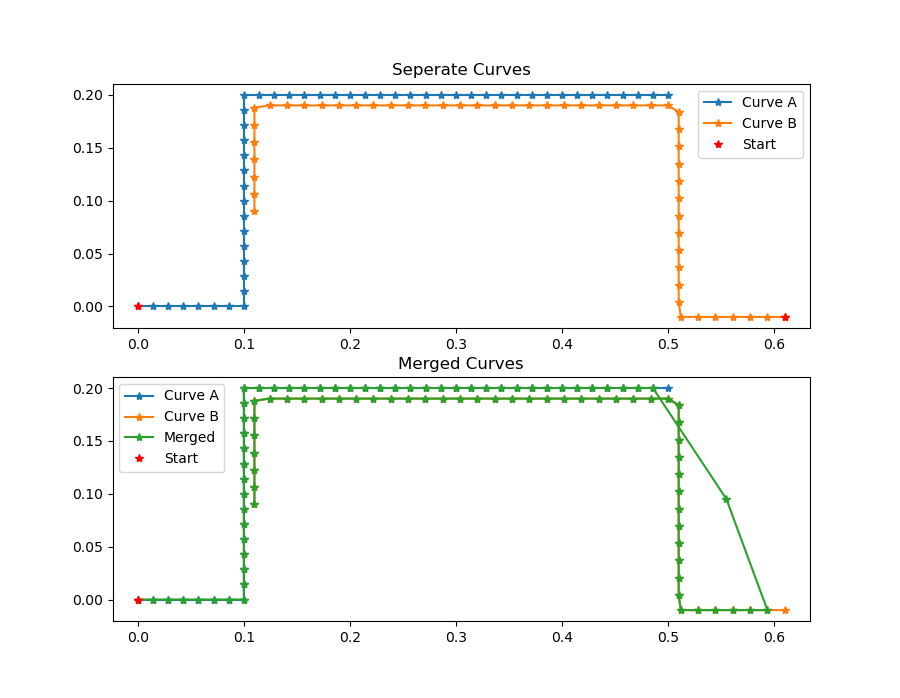
One issue when merging curves is how to handle diverging curves, meaning two curves that overlap in the middle and then diverge into different directions. The given algorithm will use the closest neighbor information to find a suitable interpolation. Each point of the to curves will be considered and this the divergent path with the most points will ultimately be dominant. Below are some examples of merged diverging curves. 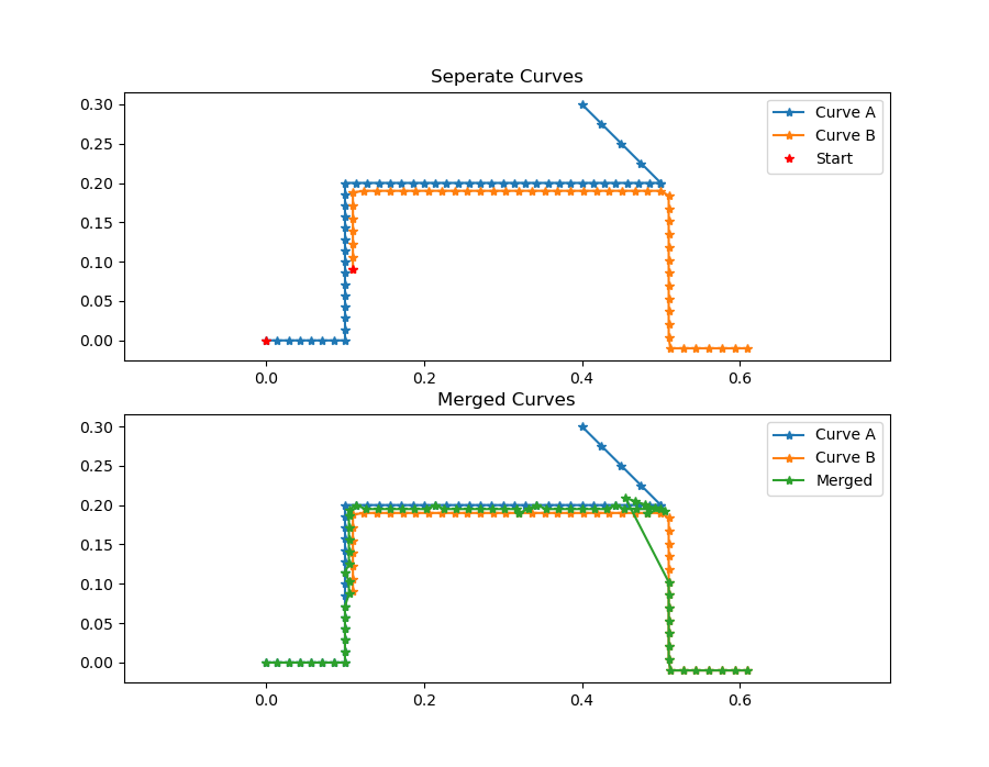
If it is unclear or undefined which one of the two given curves is the starting curve, it is determined by calculating the distance of both possible starting points to the other curve. The one starting point with the larger distance is taken as the starting point for the merged curve. This calculation is optional and can be switched on / off by the user when calling the merge curve function.
Calculating the enclosed area of a curve is equal to calculating the area of a polygon. This equality holds, since the curves in CVB are represented by points and linear interpolation between them. As a side note, the approaches described in this section do not work for other representations such as Bezier-Curves.
Below are some examples of different types of curves, sorted from simple to difficult to calculate the enclosed area. 
Basic geometric shapes have defined formulas to calculate their area and are therefore easy to calculate. Convex curves can be simply divided into triangles and the area then calculated as the sum of the inner triangles. This approach does not work for non-convex curves however.
Searching for area of a polygon or non-convex polygon one may come across the definition of a simple polygon. This is a polygon that is not self intersecting and not self overlapping. In CVB only the area of simple polygons can be properly calculated. The implemented algorithm is the shoelace algorithm which allows to calculate the area fast, but does not check if the polygon is actually a simple polygon. To check if a curve is a simple polygon the sum of inner angles can be calculated. If and only if the sum of the inner angles is equal to (p-2)*180, where p is the number of points in the polygon. This check is not part of the enclosed area function to save computation time.
The general idea of the shoelace algorithm is to calculate the area of triangles between two consecutive points of the curve and the origin (which is the point (0,0)). While adding up the sum of these triangles would be incorrect, the algorithm does consider sweeping direction between the two points of the curve. and thus does add and subtract triangles to find the correct enclosed area of any curve, as long as the curve does not intersect itself.
In CVB, the implemented algorithm will close the given curve, meaning that if the first and last point in the provided curve do not match, the curve will be closed between first and last point.
![]()
For high precision applications (e.g. pick and place), images acquired by line scan cameras have to be calibrated. There are two issues which have to be considered: First of all errors due to lens distortion and second the direction of the movement of the camera.
The following sections describe the theory behind the calibration and give a guidance how to calibrate with CVB.
The main part of the line scan calibration is the correction of errors induced by lens distortion (see Figure below). These errors can be approximated by a 3rd order polynomial.

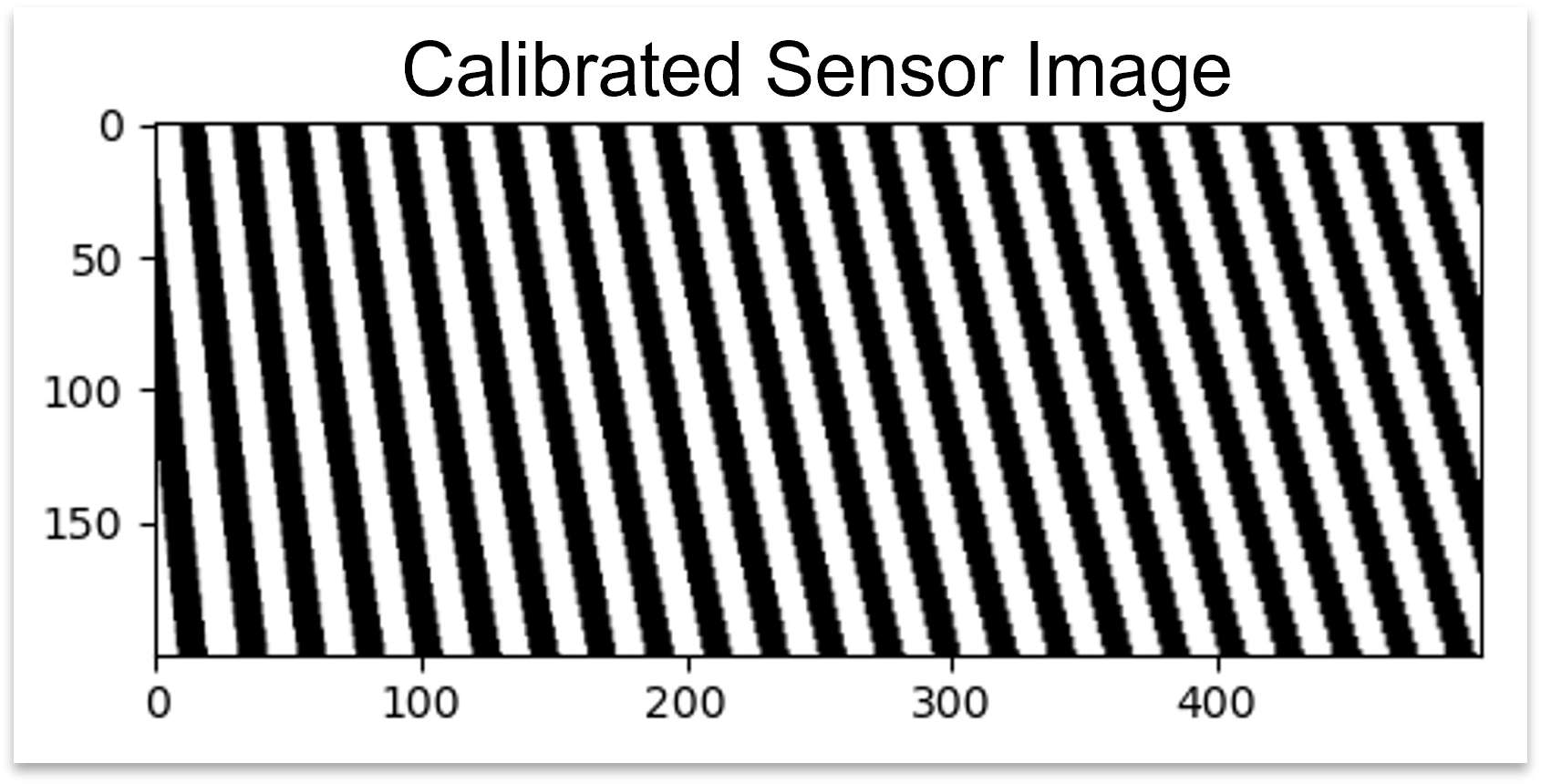
For the estimation of the correction parameters a pattern with alternating black and white stripes where the width of the stripes is known can be used. After the application of the correction, coordinates in the direction of the sensor line are metric. In order to get quadratic pixels, i.e. x and y have the same units, also the direction of movement has to be calibrated by a scaling factor. Therefore two markers circularly shaped with known position can be used (see dots in Figure below). Note, that for the calibration there can be used two separate acquisitions, one with the markers and one with the stripe pattern.
The correction parameters will be stored in the CVB NLTRANSFORMATION object and are described in Non Linear Transformation Functions in the Foundation Library.
With the line scan calibration mixed coefficients are not considered and thus zero. If the direction of the sensor line is x, the transformation is given by the following formulas. The x coordinates are corrected by a 3rd order polynomial and the y coordinates are scaled by a factor:


where
x: pixel position in x (column),
y: pixel position in y (row),
a1-a10: coefficients in x
b9: scaling factor,
x' and y': transformed x and y coordinates.

For the direction of the sensor line in y it follows:


Getting points for calibration of movement
For the calibration of the camera movement, an image of two markers circularly shaped has to be acquired. The distance between the markers in world coordinates has to be precisely known. With CVB function CVFGet2PointsForCalibrationOfMovement the user can extract the markers from the given image. Internally the CVB blob tool is used for the detection of the markers. If more than two blobs are found, the outermost blobs (most proximate to the edges of the image) are used.
Detecting edges of stripe target
To calibrate the camera itself an image of a pattern with alternating black and white stripes has to be acquired. Here, also the width of the stripes has to be precisely known and be given in the same units as the distance between the markers. CVB function CVFDetectEdgesOfStripeTarget detects the edges from the calibration pattern. Internally the CVB Edge tool is used for the edge detection.
Calibration
If both - pixel position of the markers and of the edges - are successfully identified by the tools described above, the user can start the calibration with CVB function CVFCreateLineScanCalibration. For the calibration some configuration parameters (e.g. number of maximum iterations, stopping criterica for the non linear solver, etc...) can be set. The user can also set the desired pixel size for the transformed image. The calibration parameters are stored in a CVB NLTRANSFORMATION object and can be applied using function CreateNLTransformedImage.
Image Processing functions for Filtering
The Foundation package provides functionality for various frequently used filters in image processing.
These filters are normally used for preprocessing of images to achieve better results in the image analysis.
What is a morphological operator?
Morphology is the study of form. With morphology it is possible to use knowledge about the form of images in order to detect several parts of the image.
For example the knowledge of the form of interference can support efficiently the elimination of fault.
The local erosion and dilation operators are the base morphological operators.
All morphological operators are local operations, that have to work with a structuring element.
The structuring element is a user-defined operator mask, that slides over every pixel of the image and determines the region of influence of the operator.
When to use morphological operators
Erosion is useful for
Theory of Morphological Operators
The structuring element (image 3 x 3) is dragged pixel per pixel over the image and the input neighborhood, that is covered by the mask, determines the new pixel in the output image.
1. Erosion
When the erosion operator is used the current pixel will be set to true only if the mask completely overlaps with the " 1 - region" of the input image.
Otherwise the current pixel is set to "0".
The image below shows the deletion of the region's boundary.

(a) Input image, (b) Structuring element, (c) Output image
The erosion operator chooses the smallest value from a sorted sequence of neighbouring pixels.
Therefore the darker regions become larger at the expense of the brighter regions (please see the image below).

2. Dilation
The dilation operator adds pixels to the borders of the regions.
Consequently the image object gets bigger.

(a) Input image, (b) Structuring element, (c) Output image
The erosion operator chooses the maximum value from a sorted sequence of neighboring pixels.
Therefore the dark regions become bigger at the expense of the brighter regions (please see the image below).
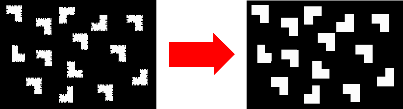
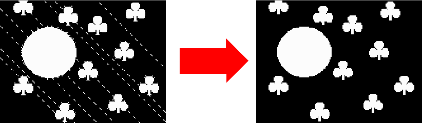
3. Opening
The opening operator consists of two morphological operations, erosion followed by a dilation (please see the images below).

(a) Input image, (b) Erosion from (a), (c) Result: Dilation from (b)
Frayed object borders are smoothened and small structures like pixel noise or small lines are supressed (please see the images below).
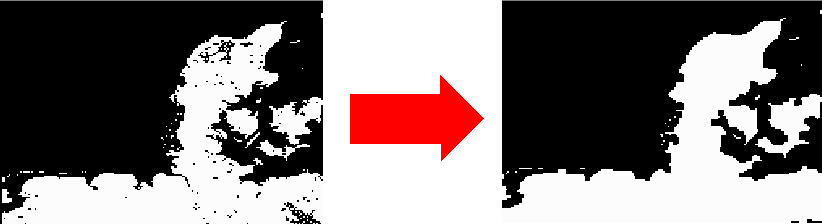
4. Closing
The closing operator consists of two morphological operations, dilation followed by erosion.

(a) Input image (b) Erosion of (a), (c) Result: Dilation of (b)
Small holes in the object's borders are closed (please see the images below).
Description
Here you can see the effects of the different morphological filter operations:
MM_Custom, MM_Square, MM_Rect, MM_Cross, MM_Circle, MM_Ellipse).For that purpose the different mask types have been applied under the different operations on the same image:

The custom mask that has been used for the MM_Custom setting is this:

The following table presents the results:
| Erode | Dilate | Open | Close | |
|---|---|---|---|---|
MM_CustomSize 16x16 Offset (8,8) |  |  |  |  |
MM_SquareSize 15x15 Offset (7,7) |  |  |  |  |
MM_RectSize 7x15 Offset (3,7) |  |  |  |  |
MM_CrossSize 15x15 Offset (7,7) |  |  |  |  |
MM_CircleSize 15x16 Offset (7,7) |  |  |  |  |
MM_EllipseSize 7x15 Offset (3,7) |  |  |  |  |

CVFoundation DLL provides Foundation Image Manipulation functions for
CV Foundation provides functions for converting and scaling images.
There are two flavors of functions that perform conversions of (multi-planar) images between two data formats:
The ConvertToXXX and the ScaleToXXX functions (where XXX stands for a short description of the target format).
Both flavors differ fundamentally in the way the conversions are performed (which in turn depends on whether conversion is done into a format with higher bit-depth or lower bit-depth):
Dst = Dstmin + n * (Src - Srcmin) with n = (Dstmax - Dstmin)/(Srcmax - Srcmin)For scaling from floating point to integer formats, the full range of values in the floating point image is automatically determined before the scaling takes place.
Scaling to floating point format converts the input image to a floating point image with pixel values ranging from the specified minimum to the specified maximum value.
Not all combinations of source and target format are currently possible!
The following table gives an overview of the currently supported scaling and conversion combinations:
| Function | 8 bits per pixel unsigned | 16 bits per pixel unsigned | 16 bits per pixel signed | 32 bits per pixel signed | 32 bits per pixel float |
|---|---|---|---|---|---|
| ConvertTo8BPPUnsigned | (X) | X | X | X | X |
| ConvertTo16BPPUnsigned | X | (X) | - | - | X |
| ConvertTo16BPPSigned | X | - | (X) | - | X |
| ConvertTo32BPPSigned | X | - | X | (X) | - |
| ConvertTo32BPPFloat | X | X | X | - | (X) |
| ScaleTo8BPPUnsigned | (X) | X | X | X | X |
| ScaleTo16BPPUnsigned | X | (X) | - | - | - |
| ScaleTo16BPPSigned | X | - | (X) | - | - |
| ScaleTo32BPPSigned | X | - | - | - | - |
| ScaleTo32BPPFloat | X | - | - | - | - |
| Examples | |
|---|---|
| CSharp | Common Vision Blox > Tutorial > Foundation > CSharp > CSFoundationFFT ConvertToXXX |
| VC | Common Vision Blox > Tutorial > Foundation > VC > VCCorrelation and VCFFTFilter ScaleToXXX |
| VC | Common Vision Blox > Tutorial > GPUprocessing > VC > VCBenchmark |
| VC | Common Vision Blox > Tutorial > GPUprocessing > VC > VC32bitFloatingPoint |
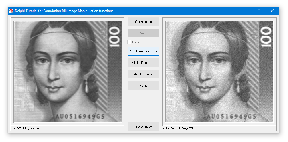
CV Foundation provides functions for manipulating Image contents.
| Examples | |
|---|---|
| Delphi | Common Vision Blox > Tutorial > Foundation > Delphi > ImageManipulation |
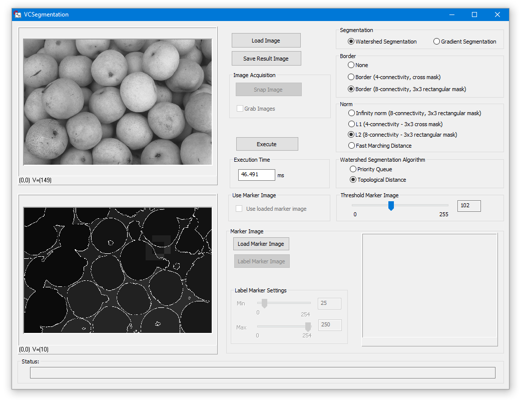
CV Foundation provides functions for Image Segmentation based on region growing with markers or watershed.
These functions only support 8-Bit images.
| Examples | |
|---|---|
| VC | Common Vision Blox > Tutorial > Foundation > VC > VCSegmentation |
CV Foundation provides functions for Image Segmentation based on region growing with markers or watershed.
These functions only support 8-Bit images.
| Examples | |
|---|---|
| CSharp | Common Vision Blox > Tutorial > Foundation > CSharp > CSGeoTransform |

Foundation LUT functions for adjusting the LookUp Table adjust an image intensity values by offering four different LUT modi.
What is a Lookup Table?
A Look Up Table (LUT) is an array indexed by the intensity value of the input pixel, containing in its entry the new intensity value of the output pixel.
The formula below describes this relationship: Dst = Values[Src] Src stands for the intensity value of the input pixel, and is used as the index in the LUT array Values for determining the output intensity Dst.
Two approaches
The Lookup Table (LUT) in the CVB Foundation Package is described in two ways:
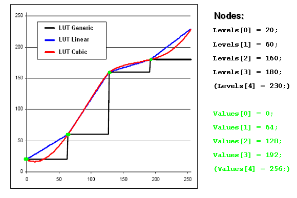
The image below shows a sample input image converted with the three LUT functions mentioned above. 

The CVFoundation.dll contains a group of functions that may be properly described by the term "Math Helpers".
This set of functions provides functionality to easily perform calculations involving several mathematical entities that exist in 2-dimensional vector space such as angles, vectors, lines and circles, allowing you to easily calculate e.g. normal vectors, intersections and even regressions.
![]()
The CVFoundation.dll contains a group of functions for Optical Flow calculations based on Lucas-Kanade Optical Flow methods.
| Examples | |
|---|---|
| CSharp | Common Vision Blox > Tutorial > Foundation > CSharp > CSOpticalFlowLK |

These functions provide statistical information on the gray value distribution in an image.
For simple information such as average, minimum and maximum brightness and standard deviation please refer to the Lightmeter Tool.

CVFoundation.dll contains functionality for Thresholding.
| Examples | |
|---|---|
| VC | Common Vision Blox > Tutorial > Foundation > VC > VCThresholding |
CVB Foundation Package includes several useful Geometric Image Transformations and Non-Lineare Coordinate Transformations.
CVB Foundation Package includes several useful geometric image transformations for rotating, mirroring, resizing images as well as Matrix Transformations and Perspective Transformations.
Perspective Transformation:
This Perspective Transformation transforms the source image pixel coordinates (x,y) according to the following formula:
where x' and y' denote the pixel coordinates in the transformed image, and cij are the perspective transform coefficients passed in the array coeffs.
Example of a Perspective Transformation, Transformation of one cube side surface
Source image and result of the transformation:
As you can see, the surface "plane" of the right cube side was transformed as if a virtual camera would be look perpendicular onto it.
The resulting image may now be subject to further processing.
The function CalcPerspectiveTransformation is used to obtain the transform coeffcients C00 - C22 first.
In order to get these coefficients, you have to specify vertex coordinates of a quadrangle which will be mapped to a destination ROI.
After the coefficients have been calculated it is possible to transform an image with the function PerspectiveTransformImage.
In addition to the height and width of the destination image you can also set a certain offset to place the section of the transformed space you would like to see.
Introduction
Generally speaking, Coordinate Transformations are useful whenever certain characteristics of an image taken by an optical system need to be corrected.
Probably the two most common uses are
In most scenarios the total distortion is a mixture of both of these effects. For example the following image has been taken by looking sideways at the slab of an optical stand through an 8 mm C-Mount lens.
Of course the perspective distortion is obvious, but if you have a close look at the lines close to the image boundaries you may notice that the lines of the grid on the slab are not straight but bent, due to the aberration of the lens being used here.
In most cases it is possible to find a coordinate transformation that allows us to transform an image as the one seen above into one that is seen as if the camera was mounted directly atop the slab.
Modeling the Transformation
There are basically two approaches to find such a transformation:
Both approaches have their advantages and disadvantages. The "scientific" approach is the more correct one, but the models necessary to properly describe the transformation are either very complex or lack portability to other problems.
As a side-effect of their complexity, they are normally numerically expensive because they take lots of calculations to perform the transformation.
On the other hand, when using a "heuristic" approach one needs to be aware, that it is not the true distortion towards which you are fitting, but just an approximation, and the quality of the fit does not really tell about the quality of the approximation - what this means will become more obvious throughout this description.
We have chosen to introduce in Common Vision Blox a non-linear transformation (as opposed to the affine linear transformations that are possible through the Coordinate System) based on a 2-dimensional polynomial model, therefore we will now have a look at the characteristics and shortcomings of the 2nd method.
Non-Linear Transformations Through 2 Dimensional Polynomials
As pointed out in the previous section, we are using in Common Vision Blox a 2 dimensional polynomial model to perform Non-Linear Coordinate Transformations.
The selection of polynomials is of course justified by the fact that polynomials are known to be suitable to approximate any continuous and differentiable function and that we expect the unknown exact transformation function ƒ(x,y) -> (x',y') to fall into this category.
The order of the polynomial is selectable, giving us a possibility to select between the quality of the fit and the speed of the transformation.
Of course there are always two such polynomials: One transforming the x coordinate and one transforming the y coordinate.
An example for a 2nd order transformation looks like this:
x' = a1 * x² + a2 * x * y + a3 * y² + a4 * x + a5 * y + a6
y' = b1 * x² + b2 * x * y + b3 * y² + b4 * x + b5 * y + b6
All that is left to do to is to find the actual values of a1, a2, a3, a4, a5, a6, b1, b2, b3, b4, b5 and b6 by performing a fit to calibration data that minimizes the error of the polynomial transformation on the calibration data.
Now mathematics tells us that the higher the order of the polynomials we use for the approximation of ƒ, the smaller the deviation between our polynomial and ƒ becomes.
While globally speaking this is really true, we should nevertheless not take this as an indication to choose the polynomial order as high as possible.
There are numerical and logical constraints that need to be taken into account.
irst of all, the order cannot be chosen arbitrarily, because we need at least as many calibration points as we have variables to fit to.
This is kind of trivial, but nevertheless worth mentioning (by the way: The number of variables for a 2 dimensional polynomial of Order n is n+1 added to the number of variables for order n-1).
The second reason is more difficult to understand: Even though higher order polynomials give a better global approximation of ƒ, the quality of the approximation may locally deteriorate!
Why ist that? Now, polynomials of higher order tend to oscillate (in fact they do oscillate so well that even sine and cosine functions may be approximated using polynomials).
And if the length of these oscillations is about the same order of magnitude as the distance between our calibration points, all we gain from higher order polynomials is a more pronounced oscillation between our calibration points - up to the point where the transformation becomes useless because it introduces too many errors between the calibration points - even though the error on the calibration points themselves is zero or at least lower than with lower order polynomials!
To illustrate this, let's have a look at the following case: Again a camera is looking sideways at the slab of a camera stand, this time with a 12 mm lens that does not introduce such a pronounced fish-eye effect.
Thanks to the grid we can easily define a great number of calibration points on the slab - we have chosen 256, arranged in a square of 16 by 16 crossing points on the grid.
With that number of coefficients we can easily calculate polynomials of up to 14th order and have a look at the transformation:
This is the untransformed image with the calibration points shown:
The 1st order transformation looks like this. Of course this is a linear transformation that would also have been possible to describe through an appropriate coordinate system of the image.
We clearly see that the linear transformation is not sufficient to describe the distortions in the image:
The 2nd order transformation already looks considerably better, especially near the center.
There is some distortion left in the left top and left bottom corner, which we could not get rid of with a (still quite simple) 2nd order polynomial...
... but already with a 3rd Order polynomial even these flaws are gone. Judging from the looks of this result, a 3rd order polynomial would be enough to get a good transformation result.
Of course the look alone is not always sufficient to judge if a calibration is good or not - we will come back to that thought a few lines later...
We may now continue increasing the order of the polynomial without seeing much of a change at first. However at some point (about 8th or 9th order) the transformed image starts to deviate from what we have seen so far.
With 11th order, the problem already is clearly visible: The lines forming the grid have started to bend between the calibration points, which is best seen, but not limited to the squares near the image border.
With 14th order, the highest order we may achieve with our 256 calibration points, things get even weirder:
Now this looks ugly. Heavily bent lines near the borders, one of the broader outside lines has even been split in two.
But believe it or not: The error on the calibration points is not higher than it was with the 3rd order transformation!
This clearly illustrates that looking at the residual error of the polynomial fit of the calibration points does not tell us enough about the correspondence between the transformation and its polynomial approximation. To determine a numerical value for this correspondence we would need to introduce some kind of norm (e. g. sum up the difference image between the original and the result of transformation and inverse transformation...).
In the absence of such a norm, the choice of the actual order of the transformation is left to our subjective impression which order solves the task best (and of course the timing needs of your application, because with increasing order, of course also the transformations will take more time to calculate, therefore we always will have a tendency to prefer lower order polynomials).
Note: Of course it would be possible to chose a regularization approach to circumvent these problems by introducing a penalty term that penalizes higher order polynomials in the regression.
While this approach evades the problem of overfitting quite elegantly it leaves us with another problem: We would need to always calculate higher order polynomials, even if they hardly contribute.
Therefore we have chosen to leave the choice of the order to be used to the user, instead of giving the user a regularization parameter to play with...
Non-Linear Transformations in Common Vision Blox
After introducing the background information necessary to use the non-linear transformations, it's about time to talk about implementation details.
In Common Vision Blox, a Non-Linear Transformation is always represented by an object whose handle is accessible through the data type NLTRANSFORMATION.
Just like the IMG object, NLTRANSFORMATION objects are reference counted object, which means that you may use the functions ShareObject, ReleaseObject and RefCount to manage the lifetime of these transformation objects.
They may be loaded from mass storage devices or stored thereon by calling LoadNLTransformFile and WriteNLTransformFile.
The functions IsNLTransform, NLTransformOrder, NLTransformNumCoefficients and NLTransformCoefficients give you further informations about a specific transformation object.
A transformation object is always generated by a call to CreateNLTransform in which the caller provides two pixel lists that give the calibration points in untransformed and transformed 2D space.
Note that along with the transformation, the inverse transformation is at the same time, so an NLTRANSFORMATION object holds both aspects of a transformation.
By the way: Of course those calibration points should not all be aligned on a single line (in other words: They should not all be linear dependent) otherwise it may not be possible to calculate a proper transformation from them).
To apply a transformation that has been loaded or created, the functions ApplyNLTransform, ApplyInverseNLTransform (both to transform a single coordinate) and CreateNLTransformedImage and CreateInverseNLTransformedImage (to transform a part of an image) exist.
Limitations
One thing to keep in mind is certainly, that transforming complete images is a time-intensive operation.
Even with only 2nd ord 3rd order polynomials you can easily spend several 100 ms in functions like CreateNLTransformedImage.
Therefore you should consider well if you really need a transformation of the whole image, or if you can do with transformations of a few coordinates only.
The first is normally only necessary, if you need the undistorted image for further processing (like doing OCR on it).
If the aim is just the transformation of a processing result in real-world coordinates, it's normally sufficient to transform a single point.
It should also be pointed out that this kind of non-linear transformation is only a 2-dimensional one.
Let's have one more look at the slab used in the previous examples: We have performed a calibration by using calibration points that were distributed over the (2-dimensional!) surface of the slab.
If we now put a 3-dimensional object on the slab...
... and then apply the coordinate transformation that has been derived from the flat calibration points, then the result looks somehow unnatural:
This is of course because the transformation does not know or care about the 3-dimensional nature of our object on the slab and just treats the image provided for transformation as if everything on the image were the same height as the slab.
If we would have wanted the 3-dimensional object to be transformed "properly", it would have been necessary to adjust the calibration points accordingly (by using calibration points taken on the object's surface rather than on the ground on which the object is lying).
For an easy access and overview and for feasibility there are several Tutorial programs available.
All of the provided with Source code so that the user could try out first if the functionality serves for his special purpose and to see the processing time of the function.
Geometrical Transformations
Non Linear Transformation
![]()
The CVFoundation.dll contains a group of functions for Wavelet Transformations.