|
|
Common Vision Blox 14.0
|
|
|
Common Vision Blox 14.0
|

The TeachBench is a comprehensive and modular multi-purpose application that serves as:
Its focus is on:
This document consists of the following topics:
Image material for training and testing may be imported from bitmap files, video files or acquisition devices and processed using the operations offered by TeachBench prior to entering a learning database or testing a classifier.
Example project files and images are stored under:
Following file types are used depending on the project:
| *.clf | Minos Classifier |
|---|---|
| *.mts | Minos Training Set |
| *.pcc | Polimago Classification Predictor |
| *.prc | Polimago Regression Predictor |
| *.psc | Polimago Search Classifier |
| *.ptr | Polimago Test Results |
| *.pts | Polimago Search Training Set |
| *.sil | Manto Sample Image List |
| *.xsil | Polimago extensible Sample Image List |
Throughout this documentation, a few terms are going to be assigned and used with a certain concept in mind that may or may not be immediately apparent when looking at these words. For clarity, these terms are listed and defined here in alphabetical order:
Advance Vector
OCR-capable pattern recognition algorithms may speed up reading by incorporating a-priori knowledge about the expected position of the next character: For a character of a given width w it is usually reasonable to assume that the following character is (if white spaces are absent) located within w ± ε pixels of the current character's position in horizontal direction (at least for Latin writing...). Therefore it sometimes makes sense to equip a trained model with this knowledge by adding to its properties a vector that points to the expected position of the following character. In Common Vision Blox this vector is generally called Advance Vector, sometimes also OCR Vector. Note that the concept of an advance vector is of course not limited to OCR: Any application where the position of a follow-up pattern may be deduced from the type of pattern we are looking at may profit from a properly configured advance vector.
Area of Interest
The area of interest, often abbreviated as "AOI" (sometimes also ROI for "Region of interest") in this document usually means the area inside an image (or the whole image) to which an operation (usually a search operation involving a classifier) is applied. One thing to keep in mind about the concept of the area of interest in Common Vision Blox is that the area of interest is commonly considered to be an outer boundary for the possible positions of a classifier's reference point (and thereby the possible result positions). In other words: An area of interest for searching a pattern of e.g. 256x256 pixels may in fact be just 1x1 pixel in size, and the amount of pixel data that is actually involved in the operation may in fact extend beyond the boundaries of the area of interest (with the outer limits of the image itself of course being the ultimate boundary).
Classifier
A classifier is the result of the learning process and may be used to recognize objects in images. To assess a classifier's recognition performance it should be tested on images are have not been part of the training database from which it has been generated, since the classifier has been taught with these very images and a classifier test on those images would yield over-optimistic results regarding the classifier's classification quality.
Command
in the context of this description means any of the available operations represented in the TeachBench's ribbon menu by a ball-shaped button with an icon.
Density
Some tools and functions in Common Vision Blox apply the concept of a scan density to their operation as a means of reducing the effective amount of pixels that need to be taken into account during processing. The density value in the TeachBench always ranges between 0.1 and 1.0 (note that in the API values between 1 and 1000 are used) and gives the fraction of pixel actually processed. Note that the density is applied likewise to the lateral and the transverse component of the scanned area (e.g. the horizontal and the vertical component of a rectangle), which means that the actual number of pixels processed for a given density d is actually d2 (e.g. with a density value of 0.5 only 0.5*0.5 = 0.25 = 25% of the pixels will be affected by an operation).
Feature Window
is a rectangular shape that defines the area from which a Common Vision Blox tool may extract information for generating a classifier. Feature Windows are usually described by their extent relative to an image location: If the object to which the feature window refers is located at the position *(x, y)*, then the feature window is described by the parameters *(left, top, right, bottom)* which give the amount of pixels relative to *(x, y)* to include in each direction (note that left and top are typically zero or negative).
Learning
is the process of generating a classifier from a database of suitably labeled sample images (see Training). The learning process is usually not an interactive process and the only user/operator input it requires in addition to the sample database is a (module-specific) set of learning parameters.
Module
A module is a DLL that will be loaded at runtime by the TeachBench application and plugs into the user interface. Modules can provide image manipulation operators or project types - they effectively decide over the functionality that is visible and usable inside the TeachBench application. The list of currently loaded modules (along with their version numbers) as accessible through the application's "About" dialog.
Negative Instance
A negative instance is the opposite of a positive instance: A sample in an image that may (at least to some degree) look similar to an object of interest, but is not actually a good sample to train from (e.g. because it belongs to a different class or because parts of the object are missing or not clearly visible). In other words: Negative instances are counter sample to the actual object(s). It should be pointed out that negative instances are (unlike positive instances) not a necessity for pattern recognitions and not all algorithms do make use of negative instances to build their classifier. However, those algorithms that do can use the "knowledge" gained from counter sample to resolve potential ambiguities between objects.
Positive Instance
Positive instances are complete and useful samples of an object of interest in an image, suitable to train a classifier from.
Project
See Sample Database.
Radius
Some of the TeachBench modules use the definition of a radius around a location of interest for various purposes (like negative sample extraction, suppression of false positive samples, sliding inspection region during OCR operations). The definition of the radius always uses the L1 norm, not the Euclidean norm - therefore radius always defines a square (not circular!) region containing (2*r* + 1)2 pixels (where r is the radius value).
Reference Point
The reference point is also sometimes called the anchor point of a model. It is the location in the pattern relative to which the feature window is described (and relative to which some of the TeachBench modules describe a model's features in the classifier). The reference point is not necessarily the center of the object but it generally has has to be inside a model's feature window. For some algorithms the reference point is "just" a descriptive feature that influences where a result position will be anchored; for some algorithms however the choice of the reference point should be given more thought because it may influence the effectiveness of (some of) the algorithm's features (like e.g. the OCR vector in Minos).
Sample Database
The sample database is the set of images generated during the training process (see Training). TeachBench projects are usually the logical representation of that database inside the TeachBench. The database will always be saved in a proprietary format specific to the module with which the project file is being edited. Projects may also be exported to and imported from directories if module-specific restrictions are observed.
Teaching
in the context of the TeachBench means the combination of training (of samples relevant for classifier generation) and learning (of a classifier).
Training Database
See sample database.
Training
denotes the process of gathering images suitable for classifier generation and pointing out the regions inside the image that contain features or objects of interest (i.e. objects the classifier should be able to identify correctly). Effectively this can be thought of as assigning a label with (module-specific) properties to an image region.
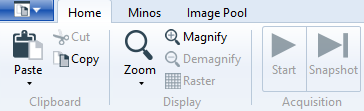
Following is a description of those parts of the TeachBench that are always available regardless of the tool modules that have been loaded. This covers the main window and the modular ribbon as well as the Image Pool which can hold any image, video or acquisition device loadable in Common Vision Blox. The Image Pool serves as a work bench on which the available operators may be applied to an image and as the basis from which the classifier training can draw - how exactly that happens depends on the module and is described in the section about the TeachBench projects.
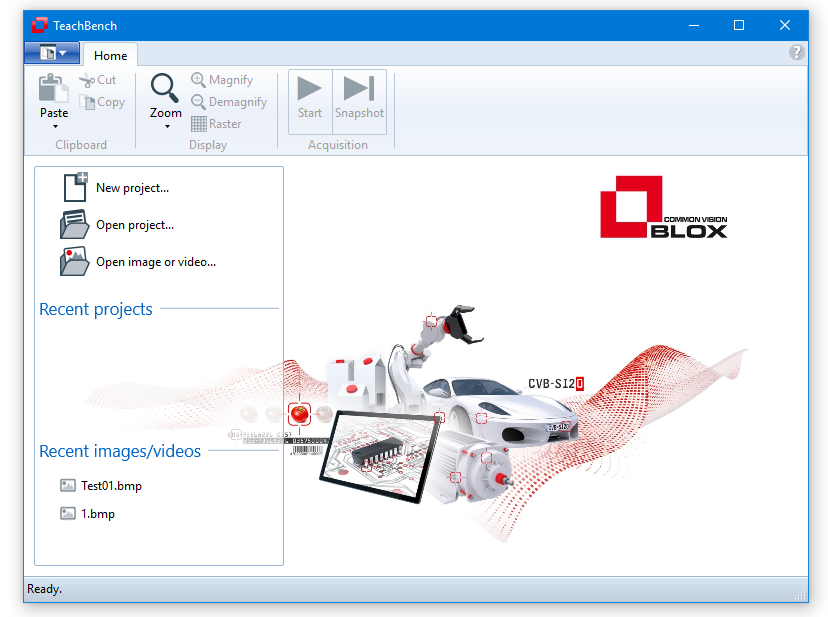
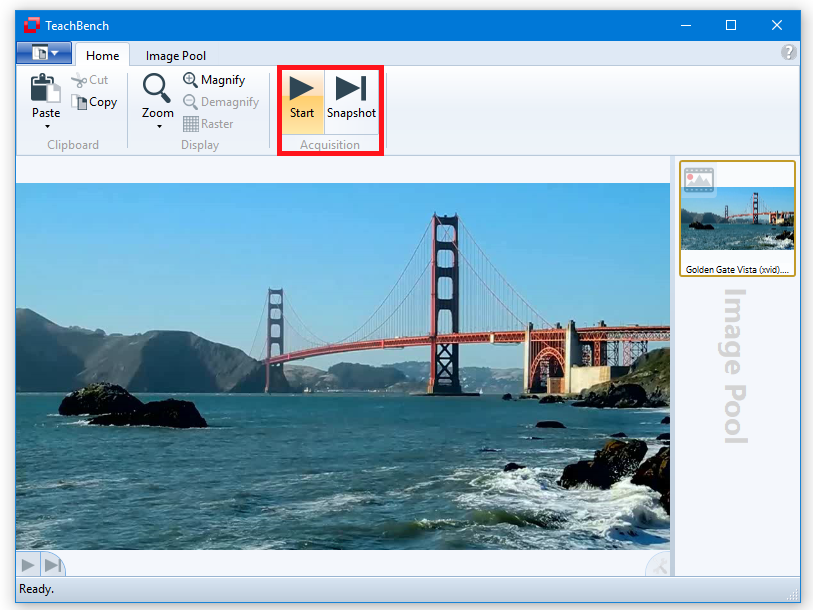
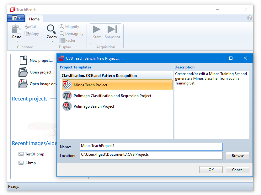
The Start View
When the TeachBench is started it shows the Start View which gives the user a chance to:
Note that these lists are cleaned (unreachable files are removed from them) every time the TeachBench starts. Entries in the lists of recently used files may be removed from the lists via the entries' context menus.
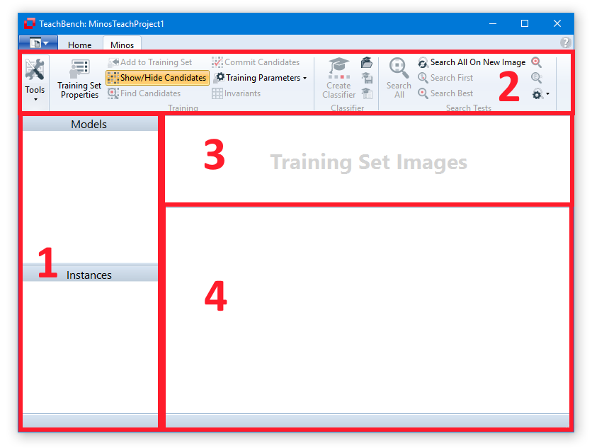
Main View
The Main View is composed of five regions, some of which might be hidden at certain times depending on the context:
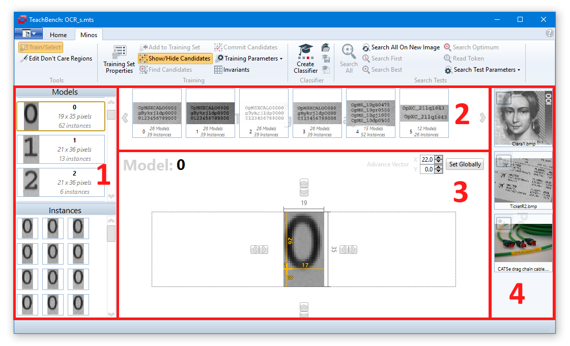
In addition to these main regions, the TeachBench user interface provides Region 5:
The options can be accessed via the File Menu. Here various general settings are displayed and can be changed. Every teaching tool has its own tab.
|
|
Values that are set here will be consistent over an application restart. Some properties might be changed via a dialog from other parts of the TeachBench and can be accessed via the Options later on.
Confirmation Settings
At some point the TeachBench might ask you for setting an option permanently. For instance, if you remove a model when working in a Minos project you will be displayed a warning.
|
|
You can check the box to not display this warning again.
These settings can be reverted from the Options Window. In this case, the option for displaying the warning when removing a model from the Training Set can be found under the tab Minos, section Confirmation. For details of the Minos options see the Options section of the specific module.
Managing and pre-processing opened images, videos and drivers
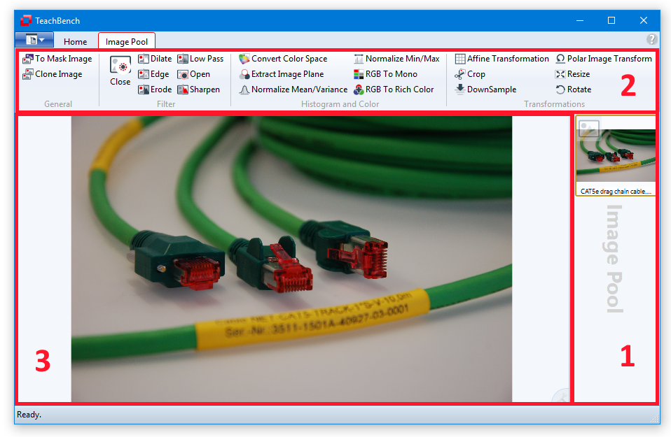
The Image Pool View consists of the Image Pool region itself at the right (1), the corresponding ribbon tab (2) and the center Editor View region (3). The Home tab is also available and provides functions regarding clipboard, display and acquisition (if a supported file is selected). The Image Pool region holds all added images, videos and drivers. Files can be added multiple times. When using the To Mask Image command, a copy of the current image is created as a mask image and immediately added to the Image Pool. Files can be added to the pool (opened) via the File Menu or by pressing F3.
In this section some exemplary work flows regarding images and videos/drivers are illustrated.
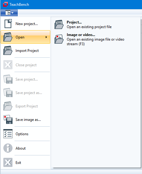
Images can be added to the Image Pool by opening them via the File Menu > Open > Image or Video.... The File Menu is located at the top left of the window. Image source files (bitmaps, videos and acquisition interface drivers) can also be opened by pressing F3.
Once an image has been opened, it is added to the Image Pool region at the right. Please note that an image is added to the pool as often as it is opened. So, one can add an identical image several times to the pool if necessary. As soon as an image has been added to the pool, it is displayed at the center Editor region. Here the mouse wheel can be used for zooming in and out of the image while holding down the CTRL key. When zoomed in, the image region can be panned by holding the CTRL key and dragging the mouse (left mouse button pressed).
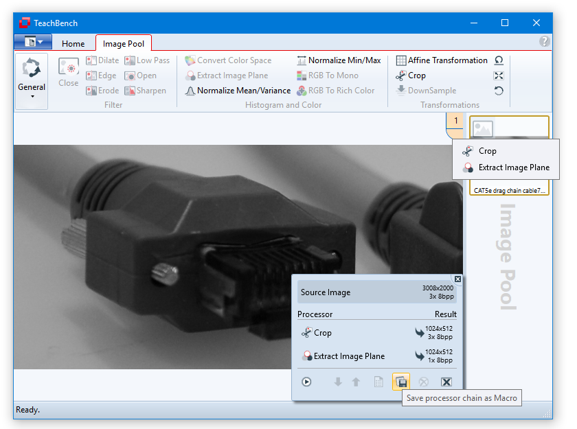
With the context menu of the Image Pool region (1) image processor stacks can be saved and loaded (applied) to a selected pool item. Images can also be saved via the context menu. Different image types are indicated by different icons. The processors of the Image Pool ribbon tab (2) are always applied to the image seen on the center Editor View Region (3). Some processors might be disabled (grayed out) in the ribbon tab depending on the currently selected image's format, size and other properties or the availability of licenses. The stack of applied image processors may be accessed via the icon at the lower right corner of the Editor View Region. Here the order in which the processors are applied and their parameters can be edited.
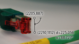
By holding down Shift and dragging the mouse (left mouse button pressed) on the display in the Editor View Region, you can bring up the Measurement Line Tool which displays distance and angle between start and end point:
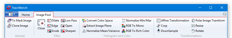
In this section, the available Image Processors will be discussed and working with Image Processor Stacks will be described. The available image processors are located in the Image Pool ribbon tab. Under General you can find the To Mask Editor command (see section Mask Editor View) and the Clone Image command.
These are:
Note that generally, the ribbon button of an operator is only enabled if the image that is currently on display in the working area is compatible with it (for example a color space conversion will not work on a monochrome image). Furthermore, some of the operators require a license for the Common Vision Blox Foundation Package. If no such license is available on the system, those operators' buttons will remain disabled.
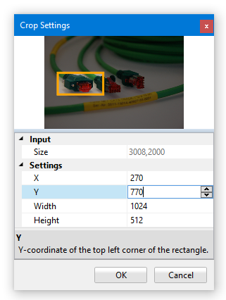
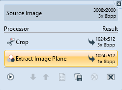
Some image processors are applied instantly to the current image by clicking the corresponding button in the Image Pool ribbon menu. Others will show a settings dialog first where various parameters may be set (when using the edit boxes in the settings window the preview will be updated as soon as the edit box looses focus). The image processors can be applied in any order and usually work on the full image. An exception is the Crop operator that can crop out a certain image area. If available for a given processor, a Settings Dialog with a preview is shown:
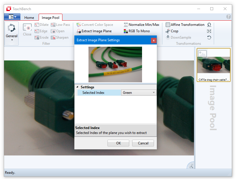
Once the image is cropped you may want to extract a single image plane (Extract Image Plane). Here, we choose the blue plane.
By confirming the operation, the image in in the Image Pool is updated. Please note that some image processors are now disabled because they are only applicable to color/multi-channel images. If at any given time an image processor is disabled, the currently selected image is not compatible (for example RGB To Mono cannot be applied to a monochrome image) - or a license for using this processor is missing.
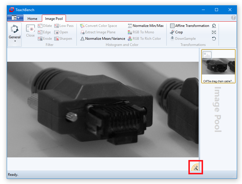
Clicking the icon in the lower right corner of the main working area all image processors currently active on this image are shown in a small pop-up window. Here the order of their application may be changed as well as the settings of each image processor (second icon from right).
The complete stack of applied processors can also be saved (to an xml file), restored and applied to other images within the Image Pool via the context menu (right-click) within the Image Pool region.
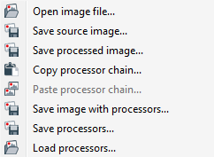
A loaded processor stack is applied automatically as it gets loaded. In order to apply a stack of processors the image has to satisfy the input restrictions based on the processors in the processor stack. For instance, the processor loading (and successive application) will fail if the stack contains a gray scale conversion or plane extraction on an image containing only one plane (monochrome image). Also a crop will not work if the target image is smaller (width and height) than the region specified in the processor settings.
This section will discuss the following Image Processors:
This section discusses the available morphological operations of the TeachBench. Morphological operations are a set of processing operations that are based on shapes (in a binary sense), the so-called Structuring Element which is applied to the input image and the pixel values of the output image are then calculated by comparing the currently processed pixel to those neighboring pixels that are part of the structuring element.
As the name implies, this tool lets you apply an edge filter to emphasize edges in an image. Edges are areas of strong changes in brightness or intensity. This image processor is represented by the following icon:
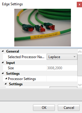
In the General section you can chose which processor you want to use. Under Settings you can chose the filter size (3x3 or 5x5) you want to use and, if the selected processor supports it, the desired orientation. Available processors are:
As the name implies, this tool filters the image with a low pass filter in order to blur (or smooth) it. If you want to blur an image significantly, you can apply this image processor several consecutive times. This image processor is represented by the following icon:
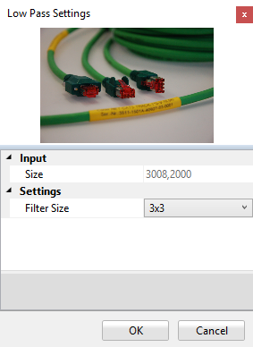
Under Settings you can chose between two different filter sizes, 3x3 and 5x5. This filter blurs an image by averaging the pixel values over a neighborhood.
Binary
With binary images it is easiest to show the effect of morphological files. Consider, for example, the following input image (generated over %CVB%Tutorial/Foundation/VC/VCThresholding):
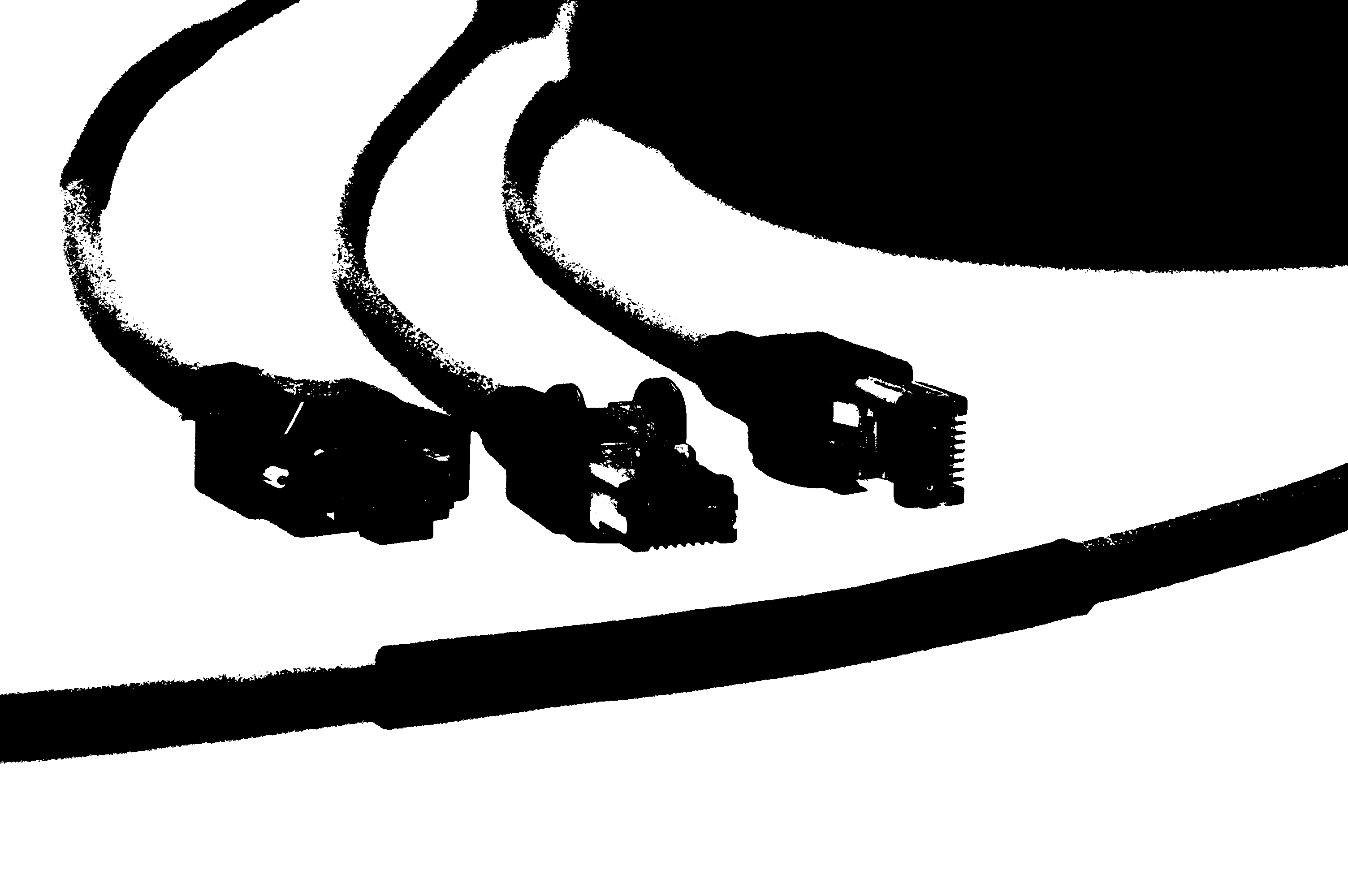
For all the operations that follow, the size of the morphological mask is defined by the parameters Mask Size Width and Mask Size Height i.e. a rectangular structuring element will be used. The mask has an anchor point whose relative position inside the mask is defined by the parameters Mask Offset X and Mask Offset Y.
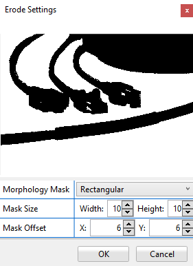
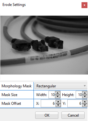
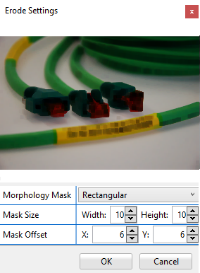
 Erosion
The morphological technique of Erosion is also known as "grow", "bolden" or "expand". It applies a structuring element to each pixel of the input image and sets the value of the corresponding output pixel to the minimum value of all the pixels that are part of the structuring element, thus increasing the size of the black areas.
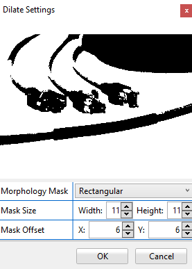
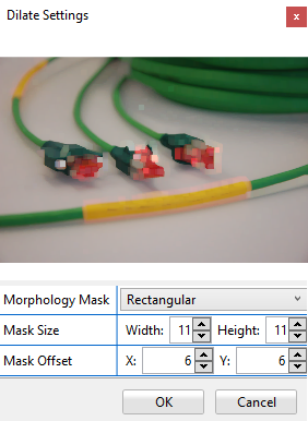
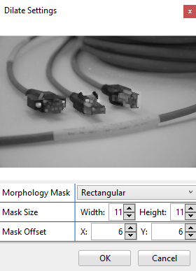
 Dilation
This method is the opposite morphological operation of the erosion. It applies a structuring element to each pixel of the image and sets the value of the corresponding output pixel to the maximum value of all the pixels that are part of the structuring element, decreasing the size of the black areas.
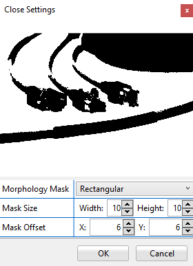
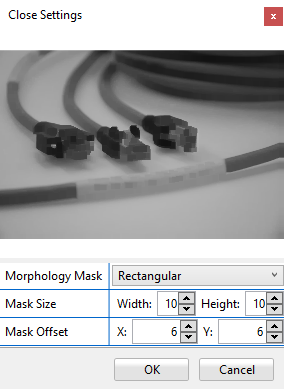
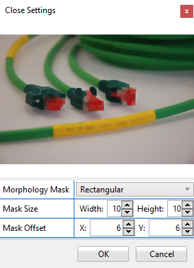
 Closing
This method first dilates the input image and then erodes it. The Closing operation is usually used for deleting small holes inside an object. Inner edges get smoothed out and distances smaller than the filter mask are bypassed.
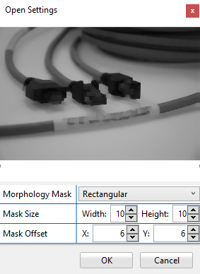
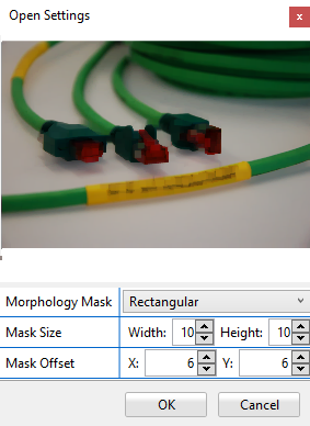
 Open
Open
This method first erodes the input image and then dilates it. The Opening operator is used for removing small regions outside of the object. Whereas outer edges are smoothed and thin bridges are broken.
Grayscale
Using morphological operators on monochrome images applies the same logic as on binary images (see above).
Color
The results are again similar for color. Here, the operator is applied to every image plane separately, which may give rise to color artifacts.
As the name implies, this tool sharpens the input image. This image processor is represented by the following icon:
It uses the following 3x3 filter kernel:

Please note: Underflow and overflow gray-values are truncated to 0 and 255 respectively. Although the function causes a visible "de-blurring" (sharpen) of images it also amplifies noise and should therefore be used with caution.
This section will discuss the following Image Processors:
As the name implies, this tool converts an image from one color space to another. This image processor is represented by the following icon:
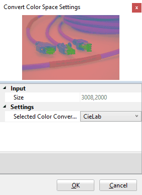
Under Settings you can select which color conversion you want to use. Available are the established conversions:
Note that the converted images are simply displayed as if they were RGB images, i.e. on YUV image the red channel represents the Y component, the green channel represents the U channel and the blue channel represents the V channel.
As the name implies, this tool extracts a single image plane from a multichannel (typically RGB) image. This image processor is represented by the following icon:
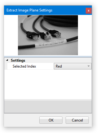
Under Settings you can select the image plane you wish to extract. The resulting image is a monochrome (1 channel) 8 bit image.
The Normalize command comes in two flavors: Normalize Mean/Variance and Normalize Min/Max. This image processors are represented by the following icons: and
and
Both commands will alter the histogram of the input image such that the output image makes use of only a selectable range of gray values (Normalize Min/Max) or that the histogram of the result image exhibits a gray value distribution with selectable mean and variance value (Normalize Mean/Variance). Both normalization modes may be useful in compensating variations in the overall brightness of image material (in such cases the mean/variance mode often provides superior results).
|
|
As the name implies, this function converts an RGB image to 8 bit mono. This image processor is represented by the following icon:
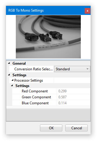
Under General, you can select the color ratio that will be used for the conversion. The Standard setting* uses:
Y = 0.299 R + 0.587 G + 0.114 B
Equal uses:
Y = 0.333 R + 0.333 G + 0.333 B
Custom lets you select different values.
This tool from the Histogram and Color section of the Image Pool ribbon menu converts an RGB image to Rich Color features. The purpose of this conversion is to enhance the color space by iteratively concatenating the available color planes. This image processor is represented by the following icon:
This function creates a nine-planar color image from a three-planar color image by adding color planes containing the information of R*R, R*G, R*B, G*G, G*B, B*B in plane 4 to 9 (normalized to a dynamic range of 0...255). Please note: Since the resulting image is no ordinary 3 channel color image, most operations cannot be performed on the resulting image (e.g. RGB to Mono).
This section will discuss the following Image Processors:
The Affine Transformation Tool from the Transformation section of the Image Pool ribbon tab launches the Affine Transformation editor which can be used for performing geometric transformations on the image. This image processor is represented by the following icon: ![]()
The available geometric transformations are:
All these transformations may be described by a 2x2 matrix:
and transformation is then defined by the following equations:
Where [ x', y' ] are the coordinates of a point in the target image and [ x, y ] are the coordinates of a point in the source image.
The four text boxes below the image at the left represent the 2x2 transformation matrix: top left a11, top right a12, bottom left a21, bottom right a22. At the right you will find a drop down box for selecting the type of transformation. Below you will find the text boxes where you can enter the desired values for the transformation operation. When using the edit boxes to modify the values please keep in mind that the preview will only update if the edit box looses focus. The available transformation operations are:
Free
If you choose the Free option, transformation matrix must be edited directly. This might be useful if a known matrix transform should be applied to the image - for all other purposes the settings described further down are probably easier to work with.
Rotation
Choose Rotation to rotate an image by any desired angle entered below the drop down box. Note that there is in fact and operator Rotate that may achieve the same effect.
Scaling
You can change the size of an image with the Scale operation. Enter the desired value in the text box below the drop down menu, once you confirm by leaving the focus of the text box you will see the changes. Values less than 1.0 result in a reduction. Enter values greater than 1.0 up to a maximum of 10.0 to enlarge the image. For example, if an image of 640 x 477 pixels is enlarged by a factor of 1.5 (50%), the result is an image of 960 x 714 pixels. Note that there is an operator Resize that may achieve the same effect.
Rotate Scale
As the name suggests, this operation rotates and simultaneously scales the image according to the entered values Degree and Scale Factor. Its result is identical to the successive application of the Rotate and the Resize operator.
ScaleXY
Same as Scale - however independent scale factors for X and Y may be entered.
 Crop
Crop
This tool allows you to crop the image and create a sub-image that only contains a part of the original image. You can either manipulate the AOI in the preview display with the mouse or change the values of X, Y, Width and Height with the corresponding text boxes.
 Resize
As the name implies, Resize allows you to change the size of an image. In the General section you can chose the desired interpolation method and whether you want to specify the desired image size in percent or in absolute pixels. The available interpolation modes are (depending on the availability of a Foundation Package license): none, nearest neighbor, linear, cubic or Lanczos. In the Settings section you can chose if you want to preserve the aspect ratio of the image.
 Rotate
As the name implies, Rotate allows you to rotate the image. In the Settings section you can specify the number of degrees by which you want to rotate the image. Here you may also select the desired interpolation algorithm. Available Interpolation algorithms are: NearestNeighbor, linear and cubic. If no Foundation Package license is available, Linear interpolation will be the only valid option.
The Polar Image Transformation is useful for unwrapping circular structures in image (for example for teaching characters that are arranged in a circle like in the example below). This image processor is represented by the following icon:![]()
The processor requires the following parameters:
This tool downsizes the image based on a Gaussian pyramid. Down Sample will cut it in half. For example, an image of 512x512 pixels will result in a resolution of 256x256 after one down sample operation. This image processor is represented by the following icon:
Note that many consecutive Upsample operation can easily bring images to a size where the memory consumption for these images becomes problematic. The TeachBench tries to handle these situations as gracefully as reasonably possible - yet simply clicking this operator 10 to 15 times in a row remains the most reliable way of rendering the application unusable or even driving it into an uncaught exception.
To create a Gaussian pyramid, an image is blurred using a Gaussian average and scaled down after that. Doing this several times will yield a stack of subsequent smaller images - a pyramid.
Videos and drivers can (just like images) be added to the Image Pool by opening them via the File Menu > Open > Image or Video... . The File Menu is located at the top left of the window. Files can also be opened by pressing F3.
Once a file has been opened, it is added to the Image Pool region. Please note that a video is added to the pool as often as it is opened, so an identical video can be processed in different ways. A camera opened by a driver is only available once due to technical limitations (an image acquisition device can usually only be opened once). Once a video/driver has been added to the pool, it is displayed at the center Editor region. The TeachBench detects automatically if a file has been opened (selected from within the Image Pool) that supports a CVB Grabber Interface and will display the corresponding controls accordingly in the ribbon section. The Start button starts the grab (playback in case of a video or EMU, acquisition in case of a driver). Snapshot captures a single image or frame. With the Snapshot button, you can go through a video frame by frame.
Similar to working with images, the mouse wheel may be used for zooming while holding down the CTRL key; the video can be panned with CTRL + dragging (left mouse button pressed). Holding down Shift and dragging the mouse while pressing the left mouse button brings up the Measurement Line Tool which displays distance and angle between start and end point.
Similar to Image Processing, compatible Image Processors can be applied to Videos and Drivers as well. The workflow and features are the same as with images within the Image Pool - for instance, processor stacks can be edited, saved and restored. The full processor stack is applied to each newly acquired image.
When the Image Pool ribbon tab is selected, you may use the To Mask Image command to create an overlay-capable duplicate of the currently visible image. Note that when the TeachBench window is displayed with its minimum size, this command is moved into a drop-down gallery named General.
|
|
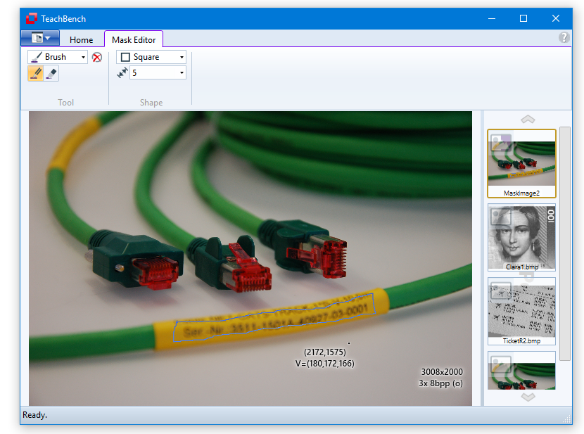
The mask editor may be used to edit a bit mask on Common Vision Blox images that have been marked as overlay-capable. This bit mask effectively hijacks the lowest bit of each pixel to define a mask that is embedded into the image data. Some Common Vision Blox tools may interpret this mask in specific way, for example it may be used by Minos to define regions where the learning algorithm may not look for features (known as "don't care" regions). The masked regions are displayed in a purple hue on monochrome images and as inverted regions in color images.
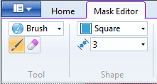
Whenever an overlay capable image from the image pool has been selected, the Mask Editor tab becomes available (whereas the Image Pool tab vanishes - the operations available for regular image pool images are usually not sensibly applicable to overlay-capable images as they will usually destroy the mask information). From the Tool section you may choose between Brush or Fill and between drawing (pencil) and erasing (rubber). In the Shape section various shapes and sizes can be selected for the brush-tip.
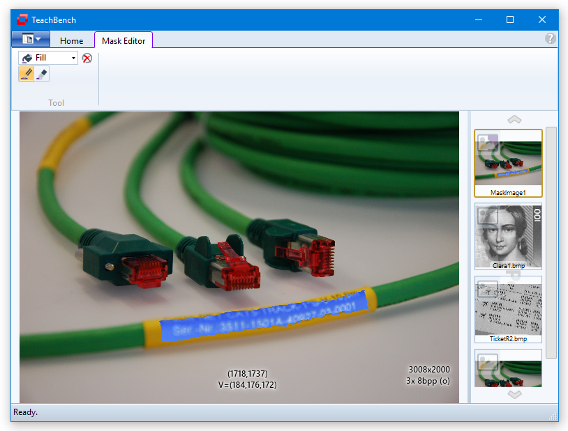
While the mask editor tab is available, you may "paint" on the image currently on display in the center region. The brush tool is useful for marking single small areas of the image. To mark larger areas it is recommendable to use first the brush tool to generate a closed line and then the fill tool. In the pictures below an area of the image has been outlined with the brush tool and is then filled with the fill tool:
The outlined area gets filled.
For an example how to use the Mask Editor to create Don't Care Regions see Don't care masks.
The main function of TeachBench is to provide an environment to work with pattern recognition projects. In these projects, patterns are taught (trained and then learned) using sample images in which the operator points out objects of interest and labels them with the information necessary for the pattern recognition tool to build a classifier. The training databases can be stored to disk (the actual format depends on the pattern recognition tool in question) and reloaded, as can the resulting classifier and (depending on the module) test results.
The Minos module for the TeachBench is intended to teach (first train then learn) patterns with the help of labeled sample images. The images which constitute the training material (Training Set Images) may be acquired from any image source supported by Common Vision Blox (i.e. cameras or frame grabbers, video files or bitmap files). A Minos classifier may contain one or more sample patterns - typical applications therefore range from locating a simple object inside an image to full-fledged OCR readers.
To train patterns, all the positive instances of the pattern(s) in the Training Set Images need to be identified and labeled by the operator. All image areas not marked as a positive instance may be considered to be counter-examples (also called Negative Instances) of the pattern. To be able to recognize an object that has been rotated or rescaled to some degree Minos may use transformations for the automatic creation of sets of models which differ in terms of size or alignment (see Invariants; note however that Minos is not inherently working size and rotation invariant an will not easily provide accurate information about an object's rotation and scale state).
Minos will use the instances and models defined by the operator to create a classifier which contains all the information necessary to recognize the pattern. When a new image (that is not part of the Training Set Images and is therefore unknown to a Minos classifier) is loaded and the classifier is applied to it via one of the available search functions, then Minos recognizes the taught pattern(s). As only the characteristics of the learned object(s) is/are stored in the classifier, the classifier is much smaller than the image information source (the Training Set Images) on which it is based. You can test a classifier directly in the TeachBench.
By switching between the learning/teaching of further instances of the pattern and testing the resulting classifier by means of the search functions in TeachBench, you can gradually develop a classifier which is both robust versus the deformations and degradations typically visible in the image and material and efficient to apply.
The sections that follow provide a guide for the steps involved in creating Minos classifiers and are divided into the following chapters:
To perform pattern recognition, Minos uses a technique which is comparable with the logic of a neural network. Patterns are recognized on the basis of their distinctive characteristics, i.e. both negative and positive instances of a pattern are used for recognition.
The criteria which distinguish between positive and negative instances are combined in a classifier in a so-called "filtered" form.
The classifier contains all the information necessary to recognize a pattern. The information is collected from various images (Minos Training Set, or MTS for short) from which the positive and negative instances of the pattern are gathered.
Once the pattern has been trained and learned, it can be recognized in other images. To do this, the classifier is used for the pattern search. We distinguish between two types of search function: pattern recognition and OCR.
Terminology
In this section the Minos specific terminology will be explained. For an overview of terms generally used in the context of TeachBench modules please refer to the Definitions section.
Model
A model in Minos is an object that is supposed to be recognized. It consists of at least one (positive) instance and is the product of the training process in Minos (see Creating Models and Instances). It is a user-defined entity. A model consists of at least one instance with its features and has a specific name. It has a specific size (region or feature window) and a reference point, these are equal for all instances that contribute to a single model.
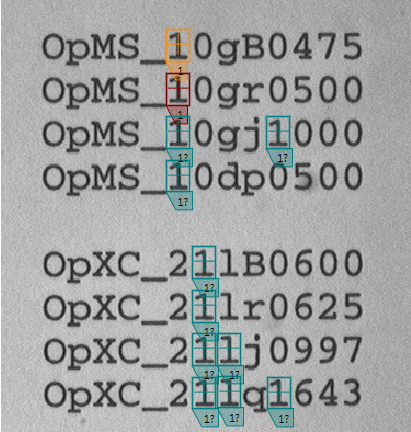
Class
A class in Minos refers to the name of the model(s). A class is made up of at least one model. If multiple models are given an identical name, they belong to the same class. For an example see the graphic above: there are different "g" character models that all form the class "g". One should be careful when selecting the positive instances of a pattern which Minos is supposed to learn; for most applications it is advised to create more than one positive instance for a pattern before testing the classifier. In the case of patterns which are difficult to recognize, you should create at least ten positive instances before assessing the performance of a classifier. In general, the more positive and negative instances are learned, the more robust the classifier will be. However, excessive numbers of positive instances which barely differ in their properties will not significantly increase the performance of the classifier. The learning and testing processes are of decisive importance for the accuracy of the classifier and thus the application's subsequent success.
Performance
Minos offers a level of flexibility and performance which cannot be achieved by pattern recognition software which works on the basis of correlations. Despite this, correlations, with their absolute measurement of quality, offer advantages for many applications. For this reason, Minos also contains an algorithm for normalized gray scale correlation. In this procedure, the pattern and the images for comparison are compared pixel by pixel on the basis of their gray scale information.
If, up to now, you have only worked with the correlation method, there is a danger that you will approach your work with Minos with certain preconceptions which may lead to unintentionally restricting the available possibilities. We therefore recommend that you read the following sections carefully to make sure you understand how to work with Minos and are able to apply this knowledge in order to take full advantage of its performance.
Pattern Recognition
Minos is extremely efficient when searching for taught patterns. Thanks to its unique search strategy, it is able to locate patterns much more rapidly and with a far lighter computing load than software products which use correlation methods. Unlike the correlation methods, these search functions can also be used to recognize patterns which differ from the learned pattern in their size or alignment.
In Minos, it is enough to learn a single classifier in order to be able to search for a variety of patterns. This classifier may be used, for example, to locate the first occurrence or the first match for the learned pattern in the image. Alternatively, you may use the classifier to detect all occurrences of all learned patterns and record these, for example, to read all the characters on a page of text.
Flexibility
You can combine different search functions and multiple classifiers in Minos. This makes it possible to develop high-performance search routines for applications such as part recognition, alignment, completeness inspection, quality control, OCR or text verification.
Easy-to-use tools and parameters allow you to control the search process, location and size of the image segment to be searched as well as the pixel density to be scanned. This means that Minos can be quickly optimized for individual application needs.
Dealing with Noise
Minos can recognize patterns with ease even in images exhibiting differing level of brightness. However, the software is sensitive to large differences in contrast of neighboring pixels (in images which contain a high level of noise or reflection). Minos is most successful when searching in images in which the shifts in contrast within the pattern are predictable and uniform. If the pattern to be learned exhibits a high level of local contrast fluctuation, or if the background is extremely varied, you will need to learn more positive instances than what would normally be the case. Using this approximation method, you can ensure that Minos will acquire the largest possible range of pattern variations which are likely to occur within your scenario. In addition, you have to adjust the values of the Minos learning parameters to be robust against a higher level noise in the image (Minimum Quality parameter, Options) or reduce the sensitivity to local contrast (Indifference Radius parameter, Options). Another way to reduce noise in an image is to pre-process the search image using the image processing functions provided by the TeachBench (Normalization, Image filtering, Applying Image Processors and sub-sections).
Coordinate System and Search Windows
Minos possesses two utilities which can be used to create "smart" search routines: flexible coordinate systems and intelligent search windows. Each pixel in an image is unambiguously defined in Minos in terms of its relationship to a coordinate system which is superimposed on the image. The coordinate system itself is flexible. That means that you can shift its origin and define its size and alignment starting from the point at which the pattern was located. This means that the position of a pattern can be described with reference to any other point. Similarly, the angle of rotation of a pattern can be expressed with reference to an alignment of your choice. Minos makes it easy to define the angle of rotation of a pattern and align the coordinate system correspondingly so that the image is normally aligned with reference to the coordinate system.
In this way, you can also search in rotated images just as if they were not rotated. When you compare this capability with correlation techniques, in which neither the scale nor the alignment of the image can be modified, you will quickly realize that Minos represents a new, higher performance approach to pattern recognition. What is more, intelligent search windows help you increase the efficiency of your application. Minos allows you to draw a rectangle as an AOI (Area Of Interest) in the search image (also see Testing a Classifier). You can specify the origins, proportions and search directions for this area. The properties of the search window are set with reference to the coordinate system, i.e. if you modify the coordinate system, the changes are also applied in the search window
In Minos it is often sufficient to create a small search window - it is unnecessary to create a large search window which demands considerable application processing time. In comparison with the search pattern, the dimensions of the search window may even be very small. It simply needs to be large enough to accommodate a pattern's reference point. Thus, it is possible to speed up the teaching and classification process significantly.
If the positioning point of a pattern is likely to be found within the region drawn in the bottom left corner, Minos need only search for the pattern in this area. Minos is able to find this pattern on the basis of its reference point.
Influence of the Coordinate System on Search Operation
For each search operation, the classifier is first transformed by the coordinate system. The coordinate system thus defines the "perspective" from which the image is to be viewed. The search direction of the Search First command is also influenced by the coordinate system: the closed arrowhead is the significant one here. Therefore, in an image in which the patterns to be found are arranged at an angle, a transformed coordinate system can considerably improve the speed of the search and the accuracy of recognition.
Quality Measure for Patterns
The Minos module of the TeachBench contains a utility named Find Candidates (see Adding Instances and Improving Models). This utility helps speed up the training process by pointing out potential instance candidates for the models that have already been trained. The potential candidates are decided upon by a correlation algorithm that runs in the background and looks through the available training set images for instances that might have been overlooked during the training process. Similarly, correlation between the original and a pattern detected during a search operation is calculated to determine an absolute quality measure of the search result (see Testing a Classifier). This measurement is performed on the basis of all pixels that have been determined to belong to the pattern during the learning phase (in other words: the correlation is only calculated over the features in the classifier, not the entire feature window).
Image Format Restrictions
Minos only works with single channel (mono) images that have a bit depth of 8. If you want to work with images that do not meet this requirement, you can use the image processors that are present in the TeachBench to make your image suitable. See Image Processing.
You can use TeachBench with Minos to teach patterns which can subsequently be searched for in new images. In this chapter we show how to teach a pattern in Minos and explain the components of the Minos TeachBench module. This section is structured along the steps of a typical work flow when creating a classifier:
When starting from scratch and no MTS (Minos Training Set) file exists, it is advised to use the Project Creation Wizard. The wizard can be reached via the File Menu > New Project....
After confirming the dialog, an empty Minos View is shown which consists of the:
When saved to an MTS (Minos Training Set) file, the only information that is being saved are the Training Set Images (3) along with the models and their instances (1). Trained classifiers are to be saved separately via the corresponding button from the Classifier section of the Minos ribbon menu (2).
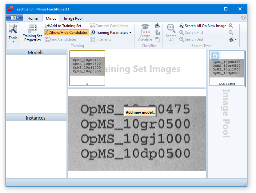
Adding images to the training set
When an image is opened, it is automatically placed into the Image Pool. Images can be added to the Training Set Images with the corresponding tool (button "Add to Training Set" at the top left ) from the Minos ribbon menu. Images can be removed from the Training Set by clicking the x-icon in the upper right corner, that will be shown when hovering the mouse over a particular image.
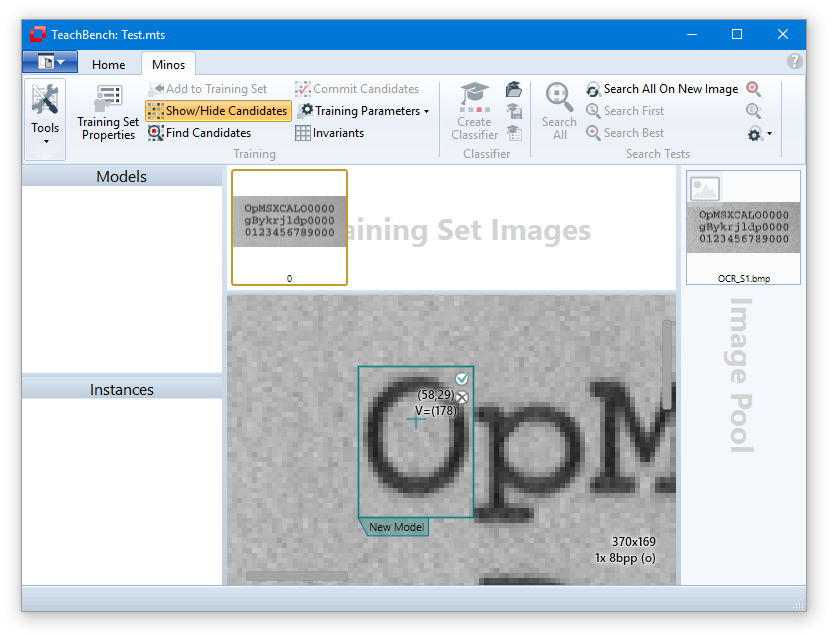
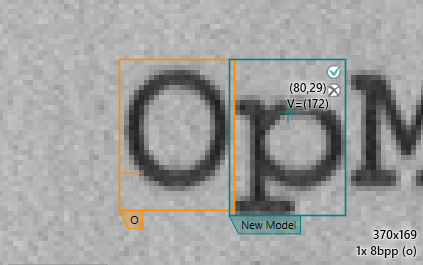
Adding an Instance
To create a new instance for a new model:
Please note: The color of the Instance Frame may be selected in the Minos options (Options).
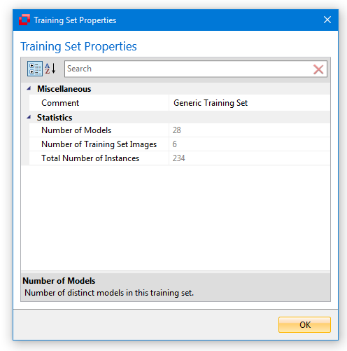
Training Set Properties
Once a training set has been created, you can review the training set properties via the corresponding button from the ribbon menu (to the left). Clicking this button will open a dialog window that shows various information regarding the currently loaded training set.
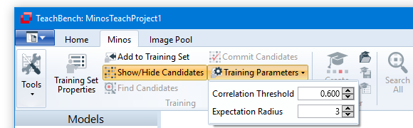
Before you actually start adding instances, you might want to review the available Training Parameters. Here you can adjust the Correlation Threshold and Expectation Radius. The values are grouped under Training Parameters in the Training Tools section of the ribbon tab. The meaning of the parameters will be explained in this section.
You may want to consider saving your training set often: The TeachBench does not currently provide any kind of Undo functionality, so any modification made to the Training Set will be committed to the data immediately and the easiest way to revert to an earlier state is to reload a saved Training Set.
Manually Adding Single Instances
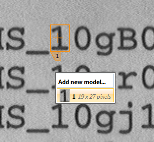
To add additional instances of an existing model, click the desired position (ideally by aiming for the reference point of the model in question) and selecting the model from the pop up window that opens. After the first instance for a model has been created, Minos is already able to approximately recognize the pattern. Thus when adding a new instance, all previous instances will be taken into consideration to best match the newly selected instance. To manually add an additional instance for an existing model it is therefore enough to roughly click the location of the reference point and Minos will try to best fit the region.
The area in which Minos tries to fit a new instance is determined by the Training Parameter Expectation Radius. The smaller the radius, the more accurate you will need to select the position of the reference point, whereas a fairly high value for the Expectation Radius may lead to the correction to drift a away to an unsuitable location (especially if only very few instances have been trained yet).
By the way: You may change the color of the Instance Frame in the Minos options (Options).
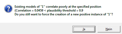
Poor Match Model
If you attempt to train an instance of an existing model that might be considered to be a poor match to the existing instances, you'll get a warning for a Poor Match to Model. In this case the correlation between the model image visible in the model list in the leftmost region of the Minos Module and the location that has been clicked is below the currently set Correlation Threshold and adding this instance to the model may decrease the resulting classifier's accuracy. If you click YES, the instance will be added to the model anyway - this is a way of passing information about the expected pixel variance in your pattern to the classifier and will effectively define a range of tolerance in which the acceptable patterns lie. If, however, you close "No" instead, the currently select reference point will be skipped and no instance will be added.
You should consider adding a poorly matching instance to the model only if the new instance actually represents an acceptable variation of the model to be expected in the image material. Note however, that if many of the variations leading to poorly matching instances are to be expected it is often a better choice to add them to new models with the same name.
In general, it is recommendable to have a large number of distinct instances for one model to grant good classification results. The instances should be distinguishable from each other. But, if successive samples do not contain much additional information, one runs the risk of unintentionally adding false information to the Training Set (for instance image noise), which may weaken the classifier. This can lead to so called Over Fitting of a classifier and can lead to many false positive results during search operations. Also, the various models should be as distinguishable as possible - select the regions accordingly.
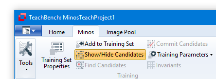
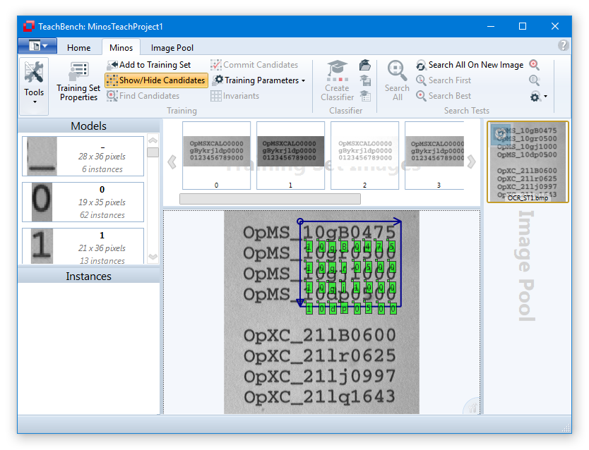
Once training has started and the first instances have been added it is possible to get automatically matched suggestions for additional instances by using the tool Find Candidates at the top left of the ribbon tab. The suggestions will be calculated for the image you are currently working on in the center Editor View Region. Before using this feature, the toggle button Show/Hide Suggestions
 has to be enabled. If Show/Hide Suggestions is enabled a search for new candidates will be carried out automatically whenever a new image has been added to the Training Set. Nevertheless it makes sense to trigger the candidate search manually from time to time - for example if new models have been added to the Training Set it's a good idea to re-evaluate the already available images.
There are three parameters in the TeachBench Options > Minos dialog (see Options) that correspond to the Find Candidates feature. These are grouped under "Candidate Search Parameters":
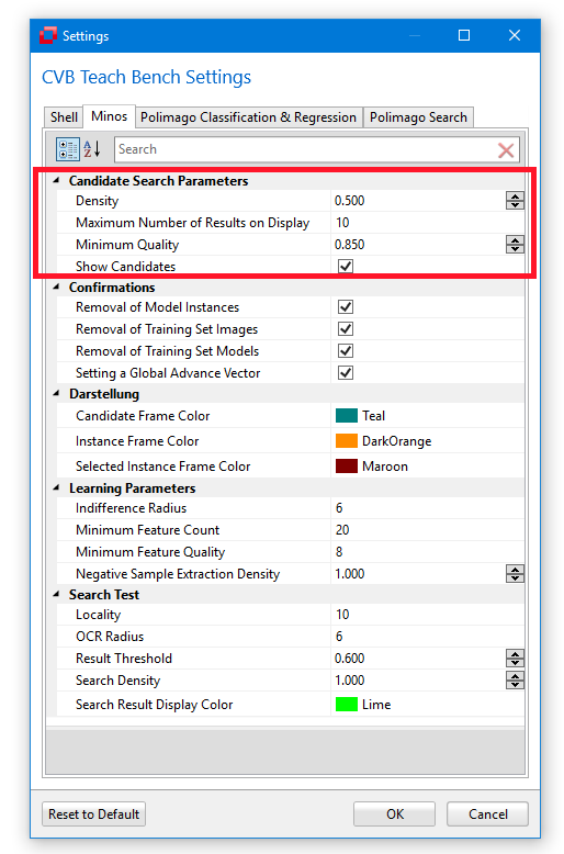
Density
The density parameter defines the search density to be used when looking for candidates (for the definition of the density please also refer to the Definitions section). Higher density values will result in a (significantly) higher search time - however the search will be done asynchronously, leaving the TeachBench as a whole available for other things. Setting the density to a lower value makes it more likely for this feature to miss a candidate in an image. While a candidate search is happening in the background, the TeachBench's status bar will show this icon:
Minimum Quality
The value of Minimum Quality is essentially a correlation threshold that determines the minimum matching level which a potential candidate must have to pop up in the image.
Maximum Number of Results
This value determines the maximum number of results that will be simultaneously shown in the central Editor View Region. Found suggestions are arranged by descending matching score so that the best ones will be shown first. If you confirm or reject a suggestion, the next one in line will be shown (if available). Limiting the number of results simultaneously on display helps preventing the Editor View from becoming too cluttered. The suggested candidates may be rejected or committed one by one to their corresponding Training Set models by clicking the respective button shown inside or next to the candidate frame. All currently visible suggestions may be added at once with the Commit Candidates button from the ribbon menu.
By the way: The color of the instance frames may be selected in the Minos options. See Options Window.
If training has already covered (approximately) all the models that are going to be needed, there is yet another feature that makes training easier, called "Next Character".
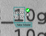
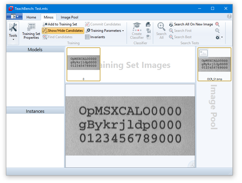
Consider the following situation: You are working with a training set that has all the characters 0-9 already trained from at least one image. Now add another image with one (or more) line(s) of numbers and manually mark the first character in the topmost row:
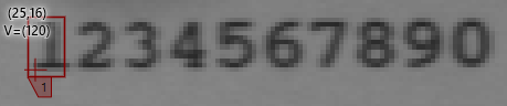
If all the subsequent characters (2, 3, 4, 5, 6, 7, 8, 9, and 0) have already been trained (and, if necessary, had their OCR vector adjusted) the remaining string can simply be trained by pressing the characters that follow in the correct sequence (in this case simply 2, 3, 4, 5, 6, 7, 8, 9, 0):
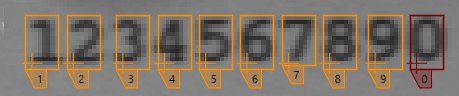
This works as long as three conditions are met:
The way the "Next Character" feature works is fairly simple: The moment you press the character to be trained next, the TeachBench will add the currently selected instance's advance vector (in this case the advance vector of the model '1') to the position of the selected instance and act as if you had clicked there and selected the model named with the character you just pressed. This means that the correlation threshold and the expectation radius (see here) will apply just as if the new instances had been trained by clicking their locations in the training set images with the mouse.
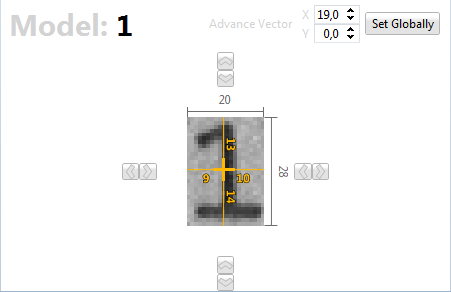
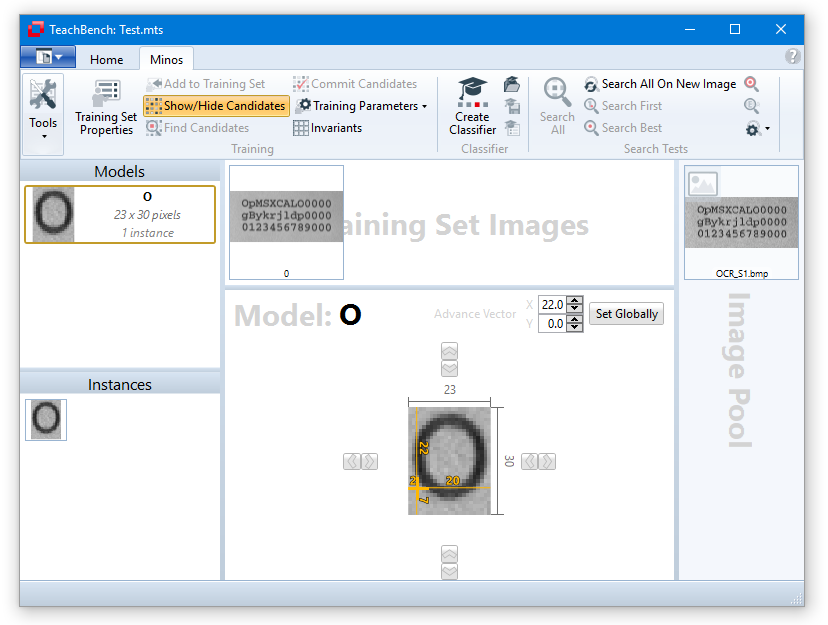
Selecting a model from the Models/Instances region (leftmost region of the TeachBench) will switch to the Model Editor View. Here you may fine-tune the feature window, move the reference point, change the Advance Vector parameter and the model name (for details on advance vectors see Defining an Advance Vector).
If there are parts of the instances you don't want to use for classification, the Mask Editor tool may be used to mask out regions in the model that are irrelevant for training (see Mask Editor View) - particularly useful when training models that have overlapping feature windows.
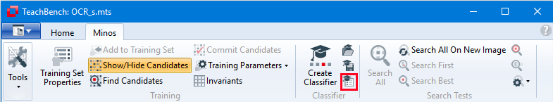
Before you start creating a classifier you should make sure that a sufficient number of instances for each model has been created (the number of created instances is shown for every model at the Models View region at the left). To train the models and instances, simply use the Create Classifier button from the ribbon menu Classifier section and save it with the Save a Minos Classifier button
Classifier Properties
When you've learned or opened a classifier, the Classifier Properties can be display via the equally named button from the Classifier section of the Minos ribbon tab. Here you can set a description and see the (read only) parameters that have been used for learning. Additionally you can find various data here like the date of creation, date of last change, model names and description.
Learning Parameters
A Minos classifier can be optimized in various ways. Besides choosing the appropriate feature window and distinct model representations during training, you should also consider the Learning Parameters Minos provides. These parameters can be found in the Minos tab of the option menu (also see Options).
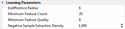
Indifference Radius
This parameter specifies the spatial distance between positive and negative instances. It defines a square whose center is located at the reference point of the positive instances. From the remaining area (pixels) outside the indifference radii of a Training Set Image, Minos may extract negative instances. In other words: The Indifference Radius defines a spatial buffer (or "neutral" zone) around positive instances where no negative instances will be extracted from. For a definition of the radius see also the Definitions section.
Setting a higher value than the default of 6 for the indifference radius may be useful if it is necessary to recognize exceptionally deformed patterns or patterns with high interference levels. In contrast, lower values result in a more precise position specification of the search results of the classifier. If uncertain, it is advisable to leave the default value unchanged.
Minimum Feature Count
Specifies the minimum number of features used for each model. Lower values result in shorter search times when using the resulting classifier whereas higher values result in increased accuracy.
Minimum Feature Quality
The minimal threshold of the contrast of a feature. Lower values result in lower contrast features to be accepted into the classifier, effectively enabling the classifier to also recognize extremely low contrast objects, whereas setting a higher value will result in features that are less sensitive to interference in the image (e.g. noise), making the classifier as a whole more resilient to noise-like effects in the image.
One should only set a higher-than-default Minimum Feature Quality if the images used for the training process possess a high level of interference (noise) and therefore a relatively high number of false negatives (patterns which are not recognized as such) are expected during testing of the classifier. Lower-than-default values are only recommendable if the aim is to recognize low contrast object ("black on black").
Negative Sample Extraction Density
This has a similar effect as the Search Density parameter (see Search Parameters). During the learning process, a grid is superimposed on the images of the training set and only the grid points will actually be checked for potential negative instances. The density of the grid is defined using the value of Negative Sample Extraction Density (for a definition of "density" see the Definitions section).
Lower values may considerably reduce the time required for the Learning Process but increase the probability that useful negative instances of a pattern may not be detected which may decrease the classification capabilities of the classifier. It is generally recommendable to use the default value of 1.0 here.
Opened (you can load one with the corresponding button from the ribbon menu ) or learned classifiers can be tested directly inside the Minos module of the TeachBench. To test a classifier, open an image that you did not use for training. Select the image you want to test with from the Image Pool by clicking it.
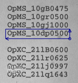
You may now either create an area of interest by dragging the mouse over the image in the center Editor View region or use the whole image by default (if no region is set explicitly). When defining an area of interest, the area can be opened in four different directions (left/top to right/bottom, left/bottom to right/top, right/top to left/bottom, right/bottom to left/top), and the direction that has been used will be indicated with two different arrows on the area of interest indicator. The area of interest is always scanned in a defined order and the direction of the two arrows defines the order in which Minos will process the pixels inside the area of interest during a search:
With Search First the* the result strongly depends on the orientation of the area of interest. Search First always interrupts a search operation if the first pattern has been found. For example in the area below the result of a Search First call will be the terminating 0 of the string.
Please note: If you can't create a search region or cannot use the Search Test tool in general, then there is either no classifier available yet or the image you are working on is not suitable for Minos to work with. See section Image Restrictions in Overview.
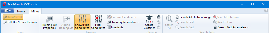
The utilities for classification tests are located at the right end of the Minos ribbon menu and are given self-explanatory names plus a tool tip that helps understanding them.
For the following images, Search All has always been used to find all matches for the models "1" and "2" with a quality threshold of 0.90 (see the Search Parameters section for details). Search results are indicated by a label in the center Editor View region.
If false positive results are found one either tinker with the threshold and the other search parameters or go back to training and refine the models and instances with more sample images and learn a better classifier.
The parameters for search tests, named Search Parameters in the TeachBench, are available via the the Search Parameters drop down menu and in the under the group "Search Test" in the Minos section (Options) of the TeachBench options.
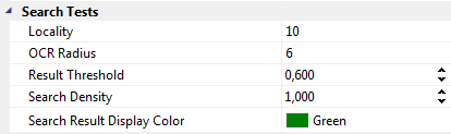
Search Density
When using a classifier on an image (or an area of interest defined on an image), a grid is superimposed on the search area and only those pixels that are part of the grid are actually checked for correspondence to one of the models available in the classifier. The density of these grid points is defined using the value Search Density (for a definition of the term Density here please see the Definitions section). Low density values reduce the time required for the pattern search considerably but increase the probability that an instance of a pattern may be missed.
Result Threshold
The threshold value represents the minimum result quality value for the pattern recognition. The higher the value, the less false matches Minos will detect but it also might miss some otherwise correct matches. The lower the value the higher will be the total number of matches Minos detects, but the chance for false positives increases as well.
OCR Radius
The OCR-Radius parameter defines the size of the OCR (Optical Character Recognition) Expectation Window when testing a classifier with the Read Token command. The expectation window is a small square, the midpoint of which is given by the sum of the Advance Vector (for the class of the last recognized character), added to the position (reference point) of that last recognized character. For details see also the sections Defining an Advance Vector and Definitions. During a read operation, the classifier only examines the pixels in the expectation window in order to recognize a character. Thus a low value for the OCR Radius permits only small deviations in the positioning point with reference to the previous character. Consequently, if there are larger variations in relative character positions a higher value for the size of the expectation window should be set (keeping in mind that too high values for the OCR radius will likely result in overlooked characters during a search).
Locality
Locality is only effective if the Search All command is used. It specifies the minimal spatial distance between matches (recognized instances). Practically speaking, if Minos recognizes two candidates within a distance lower than the given Locality (measured with the L1 norm!), it will reject the candidate with the lower quality score.
Search Result Display Color
Defines the color in which a search result will be displayed in the Main Editor View.
Another type of error which may occur are false negatives. During a search test, generally three types or errors can be identified:
False positive
An object not trained into the classifier is incorrectly identified as belonging to a class. Usually, false positives possess a significantly lower quality measure than correct search results. The identification of false positives indicates that there might not be enough positive and negative examples in the Training Set to enable the classifier to work efficiently and reliably even under difficult search conditions. So, to avoid this of problem, add the corresponding images to the contents of the Training Set (of course without marking the location of the false positive result(s)).
False negative
An object belonging to a class is not recognized as such. In other words: In this case, the search function fails to find a good match, i.e. a corresponding pattern of high quality, even though at least one is present in the image. Also in this case, the performance of the classifier can usually be improved by adding further images to the Training Set. To do this, it is necessary to use a wider range of positive instances and counter-examples. Add more images containing positive instances to the model/Training Set. Make sure that these images satisfy the framework conditions which obtain in your actual application. If you have a classifier that shows a surprising amount of false negatives during search test, it might also be a good idea to re-evaluate the images in the training set and search for instances of the class(es) involved that might have been missed during training. The "Find Candidates" command may be a useful help here (and it might make sense to slightly decrease the correlation threshold in the Minos options).
Confusing results
The result of the search function is inexplicable, incorrect or rare. Check the images in all the training sets to make sure that no positive examples have been overlooked. You can us the Find Suggestions tool from the Minos ribbon menu to aid you with finding all instances. Also see Speed Up Creating Instances - Find Suggestions.
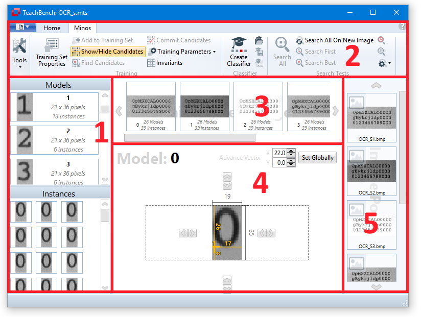
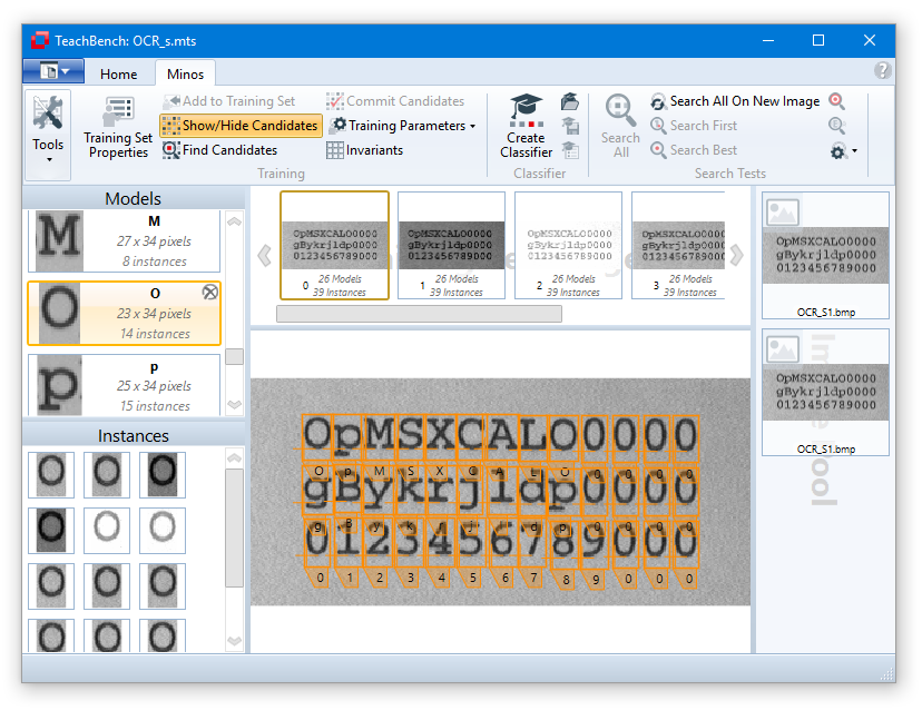
When a model is selected in the Models/Instances View at the left (1, upper part) the center Editor View Region shows the Model. The Training Set Images of the current project are shown in the dedicated region (3). All images that you added to the Training Set from the Image Pool (5) with the button Add to Training Set from the Minos ribbon menu (2) will be shown here. When you save a project as a MTS (Minos Training Set) all the Training Set Images, models and their instances are saved. Trained classifiers (CLF) have to be saved separately via the corresponding button from the ribbon menu.
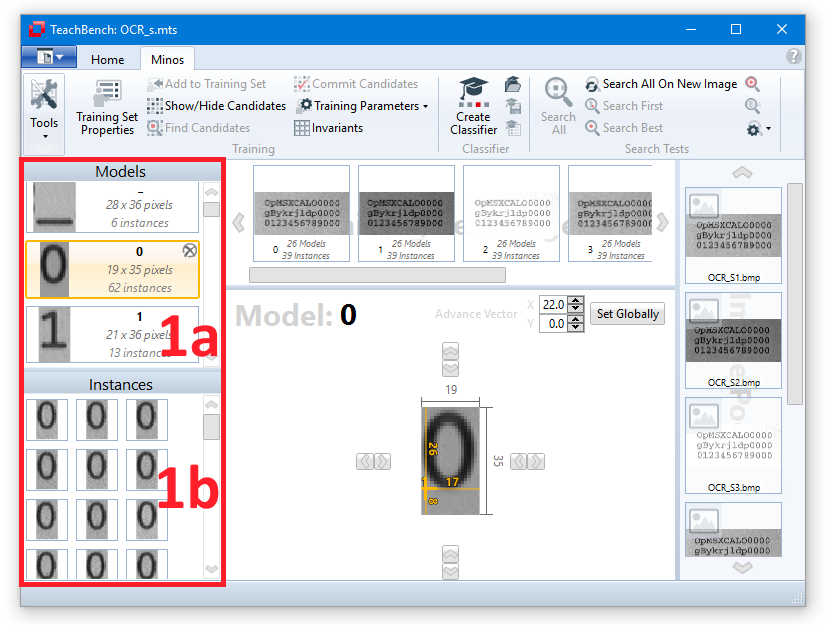
Model Region (1)
All models that belong to a Training Set are shown in the Model Region. The models are sorted ascending by their name. Under the model name you can find the size of the model region and the number of instances that have been added to the model. If you hover over a certain Model, you can remove it from the Training Set by clicking the x-icon in the upper right corner.
Model Editor View Region (2)
If you select a model from the Model Region the center Editor View will change to the Model Editor View (4). Here you can fine-tune the region for the model with the corresponding controls. You may also drag the reference point for the model, change the model name and modify the model's Advanced Vector (also see Defining an Advance Vector).
When a model is selected in the Models/Instances View (1a) the list of corresponding Instances (1b) will be shown.
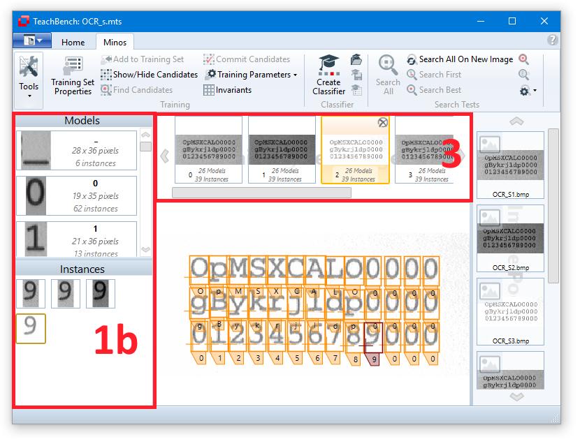
Selecting one of the Instances (1b) will select the image from which it has been extracted and display it in the Editor View region (4) with the selected instance highlighted.
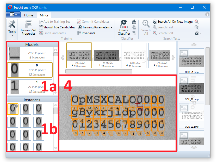
Highlighting will also work in the other direction: Selecting one of the Training Set images (in region 3) will bring up the selected image and show all the instances that have been trained from it. Clicking one of the instance frames will highlight it and select it in the Instances list (1b).
The highlighting color for the selected instance and the unselected instances may be defined in the options menu (Start menu > Options).
The following section shows you:
Minos allows you to create classifiers which recognize a pattern in more than just one rotation and scale state in one of two ways:
Adding bigger rotation/scale steps to new classes is necessary because of the way Minos works: Minos always tries to build a classifier that fits all the instances that have been added to one model. However, this is only possible if there are features common to all the instances of a trained model. Rotating models by up to ±180° will make this highly unlikely (unless the object that is being trained has some rotation-symmetric elements), making it necessary to group the instances of different scale/rotation states into different models based on their similarity (or lack thereof).
It often makes sense to combine both: If e.g. the aim is to have a rotation invariant classifier, it's recommendable to first generate the rotations up to ±180° with a higher step size (for example 10°) and then "soften" the models that have been produced by adding smaller rotation steps as well (e.g. ±3°).
The Invariants tool permits a rapid and automatic generation of the such models from existing models (see also Invariants).
Exemplary Work Flow
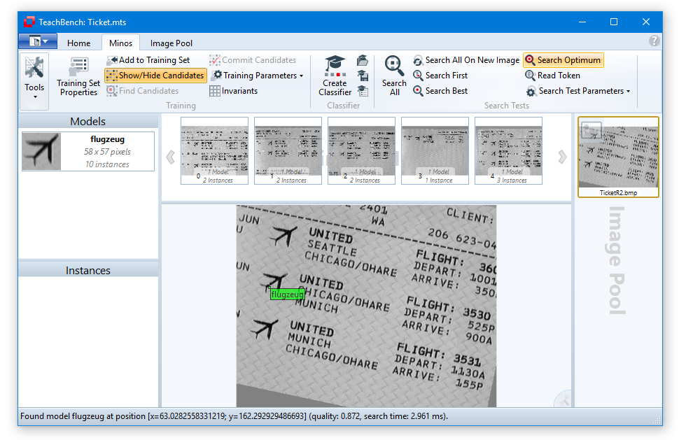
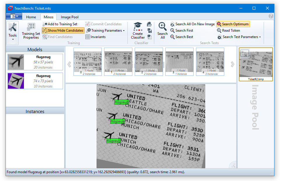
First, open the image TicketR2.bmp from the CVBTutorial/Minos/Images/Ticket sub directory of your Common Vision Blox installation. Then open the files Ticket.mts (Minos Training Set) and Ticket.clf (Classifier) from the same directory. Now press the Search Optimum button from the Search Tests section of the Minos ribbon menu. As you can see, not all instances are recognized correctly.
To improve the classifier, one may first determine the angle of the rotated object in the image TicketR2.bmp. To do this you can use the Measurement Line tool (see Image Pool View). In the original model, the line from the tip of the left airplane wing to the point at which the wing joins the fuselage is almost horizontal, about 0°. The angle measured here is approximately 11°.
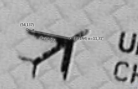
To obtain an optimum search result, is is therefore required that the model is rotated approximately 11°. To do this, click the Invariants button from the Training section of the Minos ribbon menu. Now click the two grid squares which lie immediately to the right of the origin. Since the grid has a resolution of 10, the values 10 and 20 are selected.
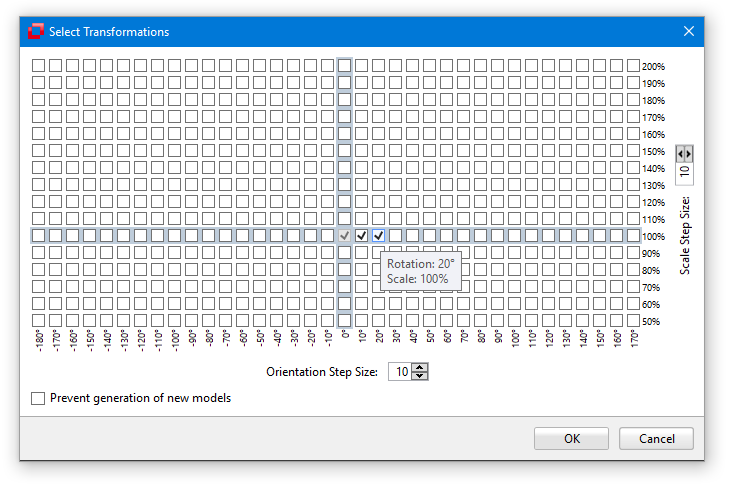
To generate the selected transformations, click the OK button. Minos will automatically generate a new rotated model with the corresponding instances.
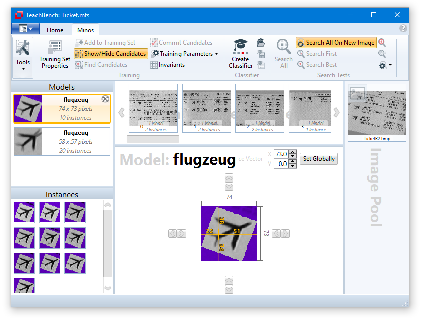
Since the content of the MTS (Minos Training Set) has changed, it is necessary to re-learn (and maybe save) the classifier.
Now test the classifier using the image TicketR2.bmp. You will see that the output quality measure is significantly higher and all three objects are now recognized.
To increase the speed of the search, reduce the Search Density parameter to approximately 500 and test the performance of the classifier again. Reduce the Search Density to 250 and see how the search speed increases. (also see Search Parameters)
The Invariants tool from the Training section of the Minos ribbon menu opens a dialog box with which additional model sets can be automatically created from existing models by means of geometrical transformations (scaling and rotation).
The Invariants tool greatly simplifies the learning of patterns which can occur in different sizes and angles of rotation (see also Rotation and/or Size-Independent Classifiers). One may simply define a single model and then use Invariants to generate additional models of the same pattern with the required scaling or rotation.
As described in Rotation and/or Size-Independent Classifiers there are situations where it makes sense to use the Invariants tool more than once on a Training Set. However please note that when using the Invariants tool repetitively, duplicate transformations will not be detected and if they do occur (e.g. by selecting +10° & +20° in the first application, then -10° and -20° in the second) they will be retained even though they do not provide useful information.
To avoid wasting storage space, it is advisable to proceed as follows when using the Invariants tool: Save the Minos Training Set (MTS) before using the Invariants tool and right before you are ready to generate your classifier (i.e. if you feel that all the necessary training has been done). Then generate the Invariants and learn the classifier from the augmented Training Set. Saving the training set is not really necessary because the generated invariants may easily be re-generated from the last saved MTS file if the transformations are known (it might be a good idea to write them into the classifer's comments, though...).
Warning: The size of the storage (and memory) space which the MTS requires after the transformations is approximately the product of the size of the original MTS multiplied by the number of transformations performed.
The Invariants tool opens a dialog box which contains a grid. Each cell in the grid corresponds to a possible orientation and size of the model in the MTS. The cells which have the size 100% and the position 0° are highlighted to provide an orientation for the user. Initially the grid is gradated in steps of 10. To obtain a finer resolution (e.g. steps of 1), you can change the step size in the box at the bottom and/or to the right of the grid matrix. The smaller steps you choose the smaller the extent to which the transformation may be performed.
In addition to its general purpose pattern recognition capabilities, specialized high-performance functions for Optical Character Recognition (OCR) have been implemented in Minos. The following chapter illustrates how to train characters in Minos, learn the classifier and test it.
The character definition process is similar to that of general purpose patterns. However, a number of additional guidelines have to be taken into account since the purpose of an OCR application is to recognize strings of characters in sequence and is thus somewhat different from "standard" pattern recognition scenario. However, these guidelines can also be applied to different applications, for example completeness control, since one significant variable for OCR, the known distance between two objects, can also be applied for different scenarios.
Before creating an OCR application you should consider the two following points:
Position
The position of a character is the pixel which represents the taught anchor point/reference point, in this case the intersection of the baseline with the extension of the left character edge. Most characters fill the entire area they occupy, but some, however, do not. Thus, for example, narrow characters such as the "i", comma character, period character and others, occupy an area which is larger than the character itself. This is particularly clear in fonts with fixed inter-character spacings.
Feature window
The feature window for all characters should be roughly identical in height, i.e. "Top", "Left" and "Bottom" should have identical values for the feature windows of the different characters. The "Right" value of a feature window describes the distance from a character's positioning point through to and including the pixel before the positioning point of the next character. In the case of fixed pitch character sets, the "Right" values of the various feature windows are also roughly identical.
Advance Vector
A character's so-called Advance Vector indicates the position at which the next character is expected, i.e. the pixel on the character's baseline which lies one pixel before the left edge of the feature window of the following character.
Expectation Window
The expectation window is a small square, the midpoint of which represents the target pixel of the advance vector. When performing a read operation (e.g Read Token), Minos only examines the pixel of this expectation window in order to recognize a character (in the TeachBench this parameter may be set in the Search Parameters, see OCR-Vector).
Don't care points
You can use the Mask Editor to mark undesired, interfering points within a feature window as areas which are not considered by Minos when learning the classifier (see also the section Don't care masks).
).
Accelerate the Creation of Instances of Existing Models
To create a high-performance classifier, you must add additional images to the Training Set and teach the classifier additional instances. A basic rule is: the more the better (also see section Terminology in Overview). To do this, open the images OCR/_S2.bmp to OCR/_S6.bmp and add these to the Training Set Images.
The images OCR/_S5.BMP and OCR/_S6.BMP contain two characters, the underscore "/_" and "q" for which no model has yet been created. Therefore, you should first create the models using the conventional procedure: left click at the desired reference point of the character (this point can be moved later via the Model Editor View) and select Add new model. Adjust the region so it fits the character properly, confirm with the green button and set a model name. Repeat this procedure for the letter "q".
To avoid having to train all characters, i.e. create all single instances, manually you can use the Find Suggestions Tool from the Training section of the Minos ribbon menu (also see Speed Up Creating Instances - Find Suggestions). In order to see the suggestions, Show/Hide Suggestions has to be enabled.
There are three parameters in the TeachBench Options > Minos that correspond to the Find Suggestions Tool , they are grouped under "Candidate Search Parameter".
Density
The density value defines the grid points on which the candidates will be looked for (for a definition of density, please refer to the Definitions section). Higher values will result in a grid with more grid points, resulting in increased time requirements for the Find Candidates run, but reducing the risk of missing suitable candidates.
Minimum Quality
The value of mminimum quality is essentially a correlation threshold that determines the minimum matching level which has to be reached before a pattern in an image is considered a candidate.
Maximum Number of Results
This value determines the maximum number of results that will be shown simultaneously in the central Editor View Region when using the Find Candidates feature. Found suggestions are arranged by descending correlation result, therefore the most promising ones will always shown first. If you confirm or reject one of the candidates, the next one in line will be shown (if available). Reducing the number of simultaneously shown candidates helps keeping the editor view uncluttered.
Creating and Testing the OCR Classifier
Create a classifier by clicking the Create Classifier button in the Classifier section of the Minos ribbon menu. When the learning process is complete, save the classifier with the corresponding button as OCR/_S.clf.
Before testing the OCR classifier, please note that, of course, all the available search utilities from the Minos ribbon may be used with an OCR-tuned classifier as well. The Read Token tool stands out because it has been specifically tailored to OCR tasks and may yield a notable performance benefit compared to the general purpose search utilities.
Read Token
The Read Token tool is the key tool for OCR applications. It operates as follows: Minos searches in the defined area of interest (note that is usually makes no sense to use this tool without an area of interest). The area of interest should be drawn around the first character's imaginary reference point. The initial search is effectively a Search First operation on the area of interest, but subsequently Minos adds the OCR vector of the found model, applies the OCR radius and analyzes only the resulting expectation window, looking for the reference point of the next character. This process is repeated until the function reaches an expectation window in which the search does not return a positive result and the function is interrupted (typically the end of a word or line).
To test the learned character set, open the image OCR/_ST1.bmp which is located in the directory %CVB%Tutorial/Minos/Images/OCR Simple/Test Images. Specify a small area of interest in the loaded image by click and drawing it with the mouse. This should be located in the bottom left corner of the first character ("O") in the first line (according to the classifier created in the previous sections). Now click the Read Token button.
If the string was not read in its entirety, enlarge the expectation window by setting the OCR radius parameter to a higher value.
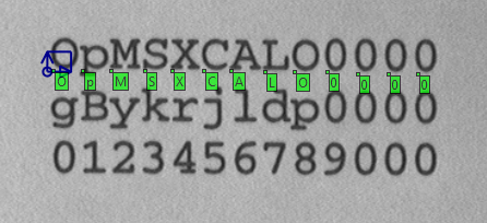
When working with fonts with fixed inter-character spacing, it makes sense to set a uniform Advance Vector for all the patterns in the MTS (Minos Training Set). This setting causes the algorithm to search for the next character at a predefined distance from the current character independently of the inter-character spacing determined by the classifier. Thus it speeds up the process and quality for an OCR application.
Because the Advance Vector was not yet defined in the preceding training example, it may be necessary to increase the OCR Radius what has a default value of 22. Please find a detailed explanation below.
To determine the distance, i.e. the measurement, for the Advance Vector, load the image OCR/_S1.bmp.
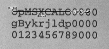
The measured distance is about 200px.
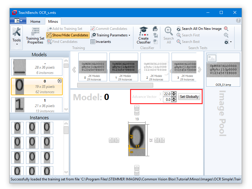
If you don't want certain parts (pixels) of the model's feature window to be used for training and classification, you can use the masking tool to point this out to the Minos learning algorithm. This works on Model images (from the model list in the TeachBench's left region) or Training Set images (form the Training Image list in the top region).
from the General tools section of the Minos ribbon tab (at the left end).Mask pixels serve different purposes depending on the object on which they have been defined:
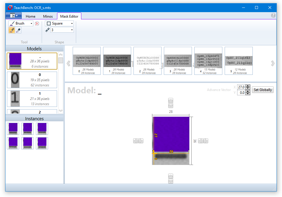
Once you finished the definition of mask regions, select the Train/Select tool from the Tools section of the ribbon menu (at the left side) so that you may continue adding models and instances.
Confirmations
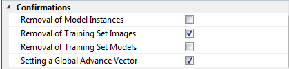
The confirmation notifications that open during various actions may be enabled or disabled here. They will (or will not if you chose so) be shown if you remove an instance, model, a Training Set Image or set the Advance Vector globally.
Consistency Check Parameters
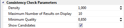
See the section Speed Up Creating Instances - Find Suggestions for a description of these parameters.
Appearance
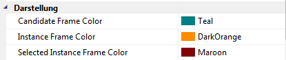
Candidate Frame Color
The color for the Instance Candidate Feature Window that will be shown when the Find Candidates command from the Minos ribbon menu is used. Show/Hide Suggestion (Show Candidates in the Options window) has to be enabled. Also see Adding Instances and Improving Models.
Instance Frame Color
The color of the instance frame that gets displayed in the center Editor View Region when a Training Set Image has been selected. Also see Image and Instance View. Every instance except the selected one will be shown with this color.
Selected Instance Frame Color
The color of the selected instance in the center Editor View Region. Also see Image and Instance View.
Learning Parameters
See the section Creating a Classifier for a description of these parameters.
Search Tests
See the section Search Parameters for a description of these parameters.
Training Parameters
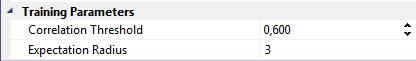
See the section Adding Instances and Improving Models for a description of these parameters.
Common Vision Blox Polimago is an image processing tool based on the Tikhonov Regularization and suitable for object/pattern recognition and classification. It is usable in two different scenarios:
As the requirements for classifier training are quite different for the two different use cases, Polimago thus comes with two TeachBench modules:
Color Format, Image Size and Classifier Restrictions
One factor to be aware of is that there is always a direct relationship between the dimensionality of the classifier and the size and number of planes of the feature window from which the classifier has been trained. As a consequence, the size and color format of the patterns used during training have to match the size and color format of the patterns in the images that the classifier will be used on. For example, if an object of 32x32 pixels in RGB color format has been trained, the search image(s) will be processed in portions of 32x32 pixels as well. Therefore the search images need to be at least 32x32 pixels in size and will have to use the RGB color format as well.
Sample Data and XSIL
The training phase, that leads to a Polimago CR classifier, involves preparing sample data i.e. images or parts of images along with the labels that go with the image content. In the context of Polimago CR, "label" means either a string label (in which case Polimago will work with discrete classes and generate a classifier for pure classification tasks) or a vector with at least one floating point value (in that case Polimago will use a regression approach). This labeled sample data is passed to a regularization engine that calculates a classifier based on a set of learning parameters (see Creating a Classifier).
Although Polimago exposes all the functions necessary for this in its API, all the steps involved in classifier creation may be carried out inside the TeachBench. The file format which Polimago CR works with and in which the data is stored, is of the so-called Extensible Sample Image List (XSIL). The DLL that caters to the creation and maintenance of this particular file format is the Sil.dll. Please refer to the documentation of the Sil.dll to learn more about the format and structure of XSIL files.
Classifier Generation
Once a Sample Image List has been created, a classifier can be learned with the corresponding tool from the Polimago CR Ribbon Menu (see Creating a Classifier). It is the user's task to provide a sufficiently high number of non-contradictory, well representative training samples for each class. What exactly a sufficient number of training samples is depends on the task - the more challenging the image material is, the higher the number of training samples should be. It is not uncommon for a well-defined classifier to require hundred or more samples per class. The selected samples should represent the various states or types of objects as comprehensive as possible.
Multiple Classes
The most basic classification task that can be solved with a linear classifier is a two-class problem. Therefore, to generate a classifier the XSIL must contain at the very least two classes. For a single class application (for example the general detection of faces) it'll be necessary to create Polimago Search Project.
If more than two classes have been added, Polimago CR will internally create one classifier per possible class pair (i.e. 3 classifiers for a 3 class problem, 6 classifiers for a 4 class problem and so forth; N*(N-1)/2 internal classifiers for N classes). This will of course have an impact on processing speed and may in practice limit the number of classes that can reasonably be added to one single classifier. Generally speaking, the classifiers generated by Polimago CR are ill-suited for a huge number of classes. From a practical point of view, anything beyond about 35 classes is questionable. Note that this applies only to the classification case - in the regression case the number of linear systems calculated only depends on the dimensionality of the labels, but not on the number of label values (number of classes). Of course, more than just one linearly independent regression label value per dimension is required to avoid singularities. Once a classifier has been created a Sample Test can be carried out in which the classifier is being tested against the content of a XSIL (of course the image and label format of that XSIL must be compatible with the classifier!). Alternatively a Leave Out Test can be calculated (for details see Testing a Classifier).
String Labels versus Vector Labels
With Polimago CR it is not only possible to classify a feature window into one of N (different) trained classes, it is also possible to calculate a regression result that expresses the currently investigated feature window as a linear combination of the (differently) labeled regression labels in the training database. This feature can be used to directly deduce a more or less continuous classification result in potentially more than just one dimension. For example, instead of training images of male and female faces, one might train the female persons with the label 1.0 and the male persons with the label -1.0. The regression results will then mostly (but not strictly!) lie in the range [-1.0 ... 1.0] and give an indication of how much a given pattern resembles either of the trained labels.This whole mechanism is not limited to scalar labels. A (theoretically) arbitrary number of dimensions may be used for these regression labels, but one should keep in mind that each additional dimension in the regression label is equivalent to adding a whole new classifier in terms of processing and memory costs. For example, one could issue two-dimensional labels with which the orientation of an object in two directions has been coded and thereby use the Polimago CR classifier to obtain a direction estimation.
Image Restrictions
Polimago CR exclusively supports images with 8 bits per pixel. These may have either 1 plane (monochrome) or 3 planes (RGB). The pixel data needs to be arranged linearly in memory (which most of the time the case when the image data comes from a Common Vision Blox supported image source).
This Polimago CR documentation is divided into the following chapters:
The goal of Polimago CR is to create a classifier and to judge its capabilities (accuracy, efficiency) with the help of the Testing utilities available in the TeachBench (see Testing a Classifier). The classifier contains all the information necessary to recognize a pattern. The information is collected from various sample images (also called Sample Image List - *.xsil) and can be saved and loaded. Based on the classification result (a class affiliation and a confidence value) a decision can be made whether or not a given sample belongs to a certain class.
The resolution and aspect ratio of samples that are supposed to be classified are crucial. Thus a robust detection or sample extraction has to be carried out before applying a classifier. One possible approach would be to first apply a classifier that distinguishes the objects from the non-objects (for example using the Polimago Search aspect of the tool) and then apply a classification on the detected set of objects in a second step.
Multi-Resolution Filter and Tikhonov Regularization
At the heart of the Polimago CR implementation there are two components:
The combination of both elements is decisive for the performance and the behavior of Polimago CR. Unlike other implementations of classification algorithms for machine vision Polimago CR users are not obliged to perform their own feature extraction prior to feeding the features to the classification engine - they can just present their image material to the algorithm, tune the MRF sequence according their requirements (choosing from a wide range of possible preferences of speed versus quality) and let the algorithm figure out the rest without having to worry about gathering features (dimensions) for the linear classifier to become flexible enough for the given task.
Class
A Class represents an object type that is supposed to be recognized. It is a user-defined entity that results from the training process and consists of at least one sample image. A class has a specific label that identifies it. A model has a specific size (region or feature window) and a reference point, these are equal for all instance that contribute to a single model.
Class Label
A class label is either a string (for classification tasks) or a vector value of arbitrary dimension (for regression tasks).
Sample
A sample is a user-defined image or region of an image that contributes to the definition of a class for Polimago CR.
Classification
The process of applying a classifier to an image or image region with the goal of assigning a class to each sample with a certain confidence. The user can set a threshold for the confidence. The aim of a classification is to categorize items, to state if it belongs to one class or another or to none of them. A classification of a sample (image) yields the result in form of a certain class label.
Regression
Unlike the classification predictor, the regression predictor does not yield a discrete result, but a value or vector values that judges the sample's relation to the learning samples in an N-dimensional continuum (N ≥ 1).
Predictor
To avoid cumulation of words derived from "classification", "Predictor" is sometimes used in Polimago CR as a synonym for "Classifier".
The main purpose of the Polimago CR Module of the TeachBench is to create and optimize a classifier that can be loaded and used in an application built on the Polimago.dll. A Polimago classification or regression predictor is unable to actually locate an object inside an image, so the detection of the points of interest to be classified needs to be done with a different approach, for example using a Polimago Search Classifer (a typical scenario would be an OCR-like application where numbers 0 through 9 need to be read; the job of actually locating the numbers inside an image could be done with a Polimago Search Classifier (which always uses just one class) and a Polimago CR predictor can then look at all the locations returned by the search classifier to identify the numbers).
As pointed out previously, two use cases exist for Polimago CR and both require slightly different training approaches:
Classifying an image into one of several classes
In this scenario, the sample image list needs to contain at the very least two classes. Therefore it will need to be applied to the known location of the object to be classified.
Regression
In this case, the sample image list will need to use floating-point-valued labels. Instead of training N different classes, the training samples are assigned target result vector values. From such a training set Polimago CR will calculate M linear systems (where M ≥ 1 is the dimension of the vector labels). Each of these systems will be able to assign a value to an input image lying roughly within the range of trained values (but not necessarily within their bounds!) and marking the sample's relative value in that dimension. With this approach it is therefore possible to assign a continuous value to the trained objects (e.g. -1.0 for the worst specimens, +1.0 for the best ones) or to assign a direction in 2 or 3 dimensions to an image (for example the estimated horizontal and vertical viewing direction of a face).
To create a new project use the corresponding command from the main menu or the start view of the TeachBench.
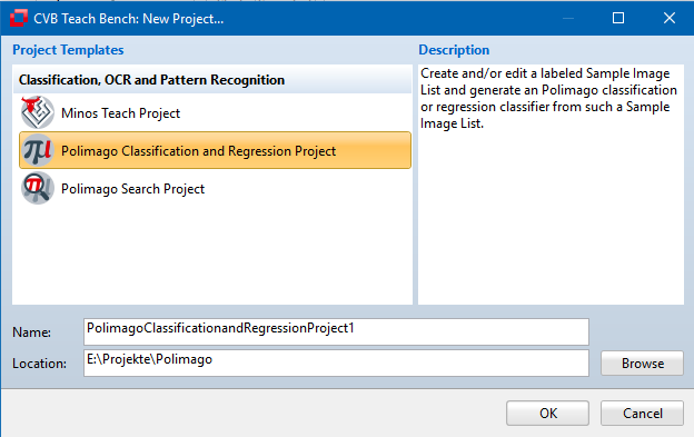
This will trigger a series of dialogs that will help you configure the sample image list properly. After the first page you'll need to chose between two kinds of labels - string or vector. This decision is essential (and immutable later on) and the right choice depends on the scenario and kind of application.
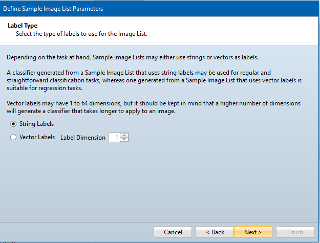
String labels are used for classification tasks while vector labels are used for regression tasks (see also Terminology). If you select vector labels you'll need to choose a dimension (between 1 and 64 - the higher the dimension, the longer the application of a trained classifier to an area of interest will take).
Next, it is necessary to configure the feature window. To make the process easier, it is possible to load an image and use it as a guide to adjust the region. Here you can also chose between working with monochromatic images (dimension = 1) or color images (dimension = 3). Besides adjusting the width and height of the object region, you can - if necessary - also modify the position of the reference point by unchecking the "center" box and set values for X and Y.
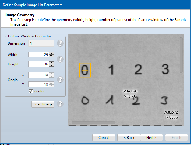
The parameters defined here become immutable properties of the sample image list that is going to be trained, so choose carefully. When in doubt, it sometimes makes sense to define the width and height slightly larger than the absolute minimum to provide some leeway for future changes. Adding additional space also may help if you plan on applying transformations to the images later on (see next wizard pages). When considering the right size of the feature window, the information in the section about the Multi Resolution Filter may also be helpful.
On the next and final page a summary of the project's settings will be given. At this point it is still possible to go back and modify the settings that have been made. Clicking "Finish", however, will close the wizard and generate an empty sample image list with the settings that have been made.
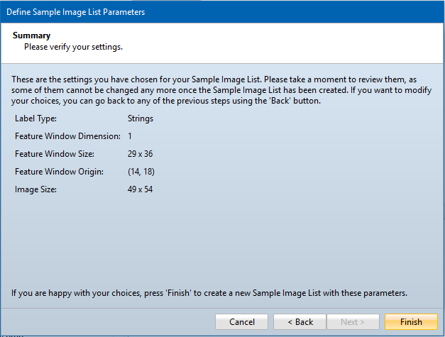
Project Properties
Once you've finished creating a project, you can review the project properties from the designated button at the left most area of the Polimago CR ribbon menu. The property view that opens will show the settings that have been made during generation of the Sample Image List.
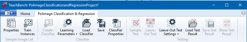
To create new models (classes), open an image in the Image Pool. When the Polimago CR (Classification and Regression) module is active and an image is selected on the pool that is compatible with the sample image list that is currently being edited (with respect to pixel type, size and number of planes) a marker tool will be displayed on the Image Pool's edit view. This marker does not belong to the Image Pool, but to the Polimago CR module and allows for the extraction of training samples.
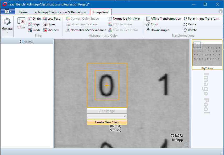
The extraction tool (displayed by default with an orange border and two buttons and a combo box underneath it) consists of 1 or two rectangles and a cross hair.
Start creating a new class by positioning the extraction tool on an object. If the project is empty and no class has been trained yet, you'll need to create a new one by clicking the button labeled "Create New Class".
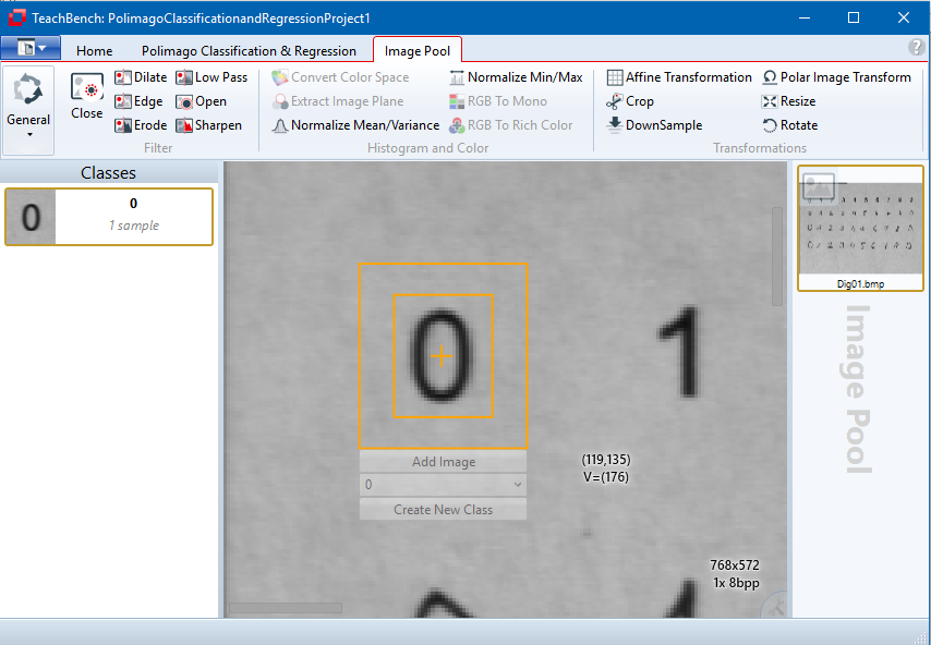
If you've already created classes and previously learned a classifier from your sample image list, the selected region will be classified on the fly as you drag the extraction tool across the image and the tool will automatically suggest a class (the combo box will update accordingly). This way you can add new samples for existing classes quickly and efficiently. Of course, the quality of these on the fly classifications heavily depends on the number of samples already in a class when creating a classifier as well as the learning parameters, so it should not be applied without double-checking it.Also, it is only possible with string labels.
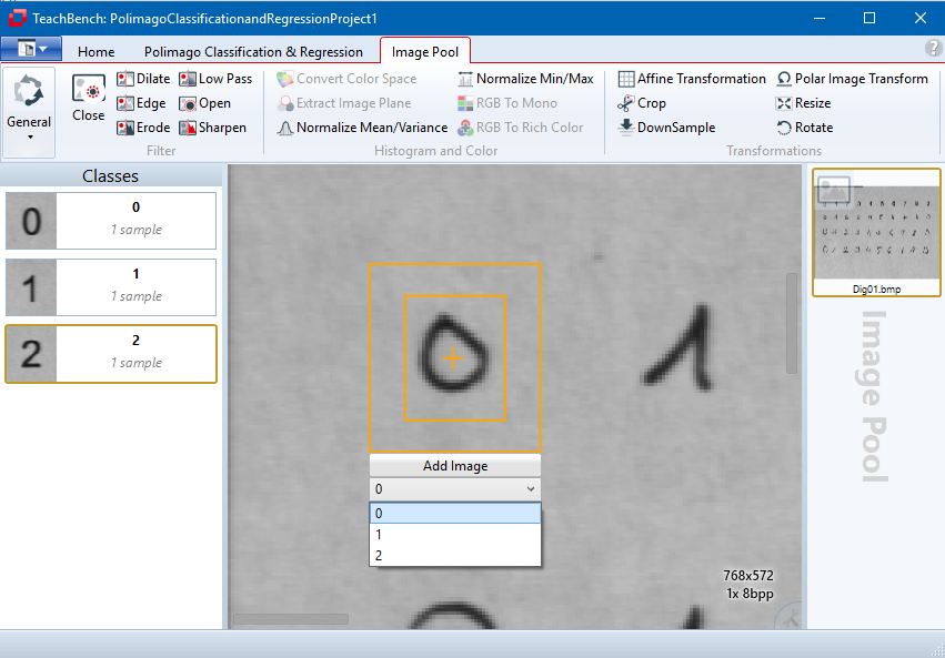
When you have done this for all classes and several images, the result may look like this:
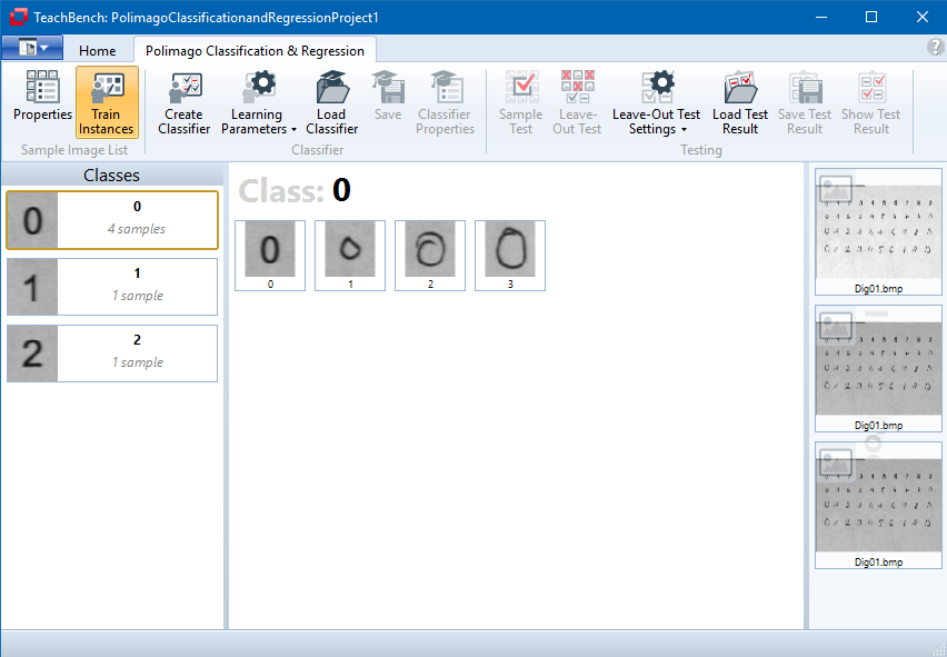
The more samples per class the better the classifier will be at the end. The next step will describe the creation of the classifier.
All classifier creation related tools may be found in the "Classifier" section of the Polimago CR ribbon.
Learning Parameters
When learning a classifier, one should have a look at the Learning parameters first (button ). The available parameters slightly differ depending on what kind of labels have been chosen during project creation (see Creating a New Project). For a sample image list that uses string labels, the following parameters are available:
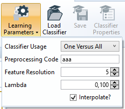
For projects that use vector labels, the Classifier Usage will be fixed to Regression.
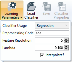
Creating and Saving a Classifier
After the Learning Parameters have been set, you can create a classifier with the designated Create Classifier button from the Polimago CR ribbon menu. Please note that, depending on your number of classes, number of samples images, project properties and learning parameters, this can take a considerable amount of time. If the classifier creation fails, an error message will be displayed in the status bar at the bottom of the TeachBench. If the classifier creation was successful, you can save it via the designated Save button from the Polimago CR ribbon menu and load it later into the TeachBench Polimago CR module or with the Polimago.dll's methods.
Classifier Properties
If the classifier creation was successful, you can review the Classifier properties with this tool (Classifier Properties button ). A property grid will show a list of classes (if applicable), the parameters that have been used during classifier creation and other, project specific, parameters like feature window size. These parameters are just for reference and cannot be changed.
The multi-resolution filter (MRF), defined by the parameter called Preprocessing Code in Polimago, is one of two parameters with the largest influence on the behavior of the resulting classifier in terms of processing speed as well as result confidence (the other important parameter being the feature resolution). It is therefore essential to tune this filter properly for a given application.
MRF and Preprocessing Codes
The purpose of the MRF is to transform the sample image data into vectors suitable for pattern classification. Evidently e.g. hand-written characters of 28x28 pixels will need a different preprocessing than surface textures of different hardwoods. Therefore the MRF can be defined and parametrized by a code string that tells Polimago how to perform the actual preprocessing. The preprocessing code that has been used for training a classifier becomes an immutable property of the classifier and will be applied likewise as search, regression, and classification operations are carried out with that classifier. The choice of the optimal preprocessing code for a given sample image list essentially needs to be determined experimentally.
The MRF is basically a sequence of filters. The image to be analyzed is fed into the first filter, the output of the first filter is fed into the second filter and so on. The output of the last filter becomes the vector that represent the input sample in the space in which the classifier operates. There are three types of filters available, p, s and a. Consequently the MRF may be described by a code-string consisting of the letters p, s and a. The string "paa" for example means that the first filter is of type p, while the second and the third are of type a. Each filter step reduces the resolution of the input by a factor of two, so that the entire MRF reduces the resolution by a factor of 2n where n is the length of the defining string. For example "paa" reduces by a factor of 23 = 8 and if the input image has width and height of 1024x512 the MRF output will just be 128x64 pixels. However, these pixels may span several images planes, so this does not necessarily imply a data reduction yet.
This resolution reduction also implies that the returned position of a result reported by such a classifier is accurate only up to ±8 pixels in this example. In other words: Any preprocessing code introduces a positional inaccuracy of ±2n.
It should also be pointed out that the input for the MRF sequence is not actually the image as it has been added to the sample image list (at least for feature resolution values ≠ 0), but the so-called Retina, whose size is determined by feature resolution and preprocessing code (see Lambda, Feature Resolution and Interpolation).
While the a and s filter (s is actually just a more sloppy but faster version of a) are being used to separate frequency components at the current resolution stage into additional image components, the p filter simply smooths over details and reduces the amount of data by a factor 4 every time it is applied. In our previous example, where there was 1/2 MB in each input image (assuming each pixel has exactly one byte), the preprocessing code paa will yield an output of only 128 kB. In other words, a preprocessing code may reduce the amount of data to be processed (and hence the processing time) by (22)m where m is the number of p characters inside the preprocessing code.
(There is also a fourth character, '+', which may occur in a preprocessing code; '+' causes Polimago to apply the MRF for the string up to the '+' plus the MRF for the entire string (without the '+' character(s)) and then concatenates both; e.g. 'aa+s' generates the feature vector for 'aa' and the feature vector for 'aas' and then concatenates both)
Deformations and Textures
From the point of view of pattern recognition, the length of the preprocessing string corresponds roughly to the (base 2) logarithm of the scale of deformation invariance or local translation invariance. This can also be viewed as some sort of elasticity of the features constituting a pattern. If the relative positions of features or structures within a pattern vary over 8 pixels distance for the samples of a given class, one will actually need a preprocessing code of length 3 at least, resulting inevitably in a positional inaccuracy of 8 pixels. This positional inaccuracy must generally be regarded as the price that has to be paid for robust recognition in the presence of deformations.
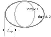
The image above shows two samples of the same class which can be generated from each other by deformations. In this case, the preprocessing code should have a length of at least n to absorb the deformation, which in turn would imply a positional inaccuracy of at least 2n pixels. An important application of this is the recognition of textures, which are patterns with a large amount of translation invariance. An oak surface remains an oak surface irrespective of the choice of the window considered. The inaccuracy of positioning is and has to be maximal. This has the following consequences:
Lambda, Feature Resolutiona and Interpolation
Lambda
Unlike its predecessor Manto, Polimago does not use discrete "decision boundary" values. Instead, the user may modify the regularization parameter (lambda) directly. As the former concept of decision boundary and the regularization parameter of the Tikhonov Regularization have no direct relationship, it is not possible to precisely map the previously used decision boundary settings to lambda values. The regularization parameter effectively controls a classifier's strictness: Classifiers calculated with a higher value for lambda will have a tendency to be better at recognizing things that were not part of the training set, while on the other hand such a classifier will be less capable of discriminating between more or less similar objects than a classifier generated with a smaller value for lambda. Therefore, the choice of lambda is ultimately a means of tuning a classifier's generalization capabilities.
Feature Resolution
The feature resolution describes the resolution in pixels (of undefined dimension - may be anything from 1 upward) of a square that makes up the classifier area. This area is also referred to as the "Classifier Retina". When generating or using a classifier, the image data to be processed is first mapped to the Retina using one of two available interpolation methods (see below), then the MRF (Multi-Resolution Filter) is applied to it. If the Feature Resolution is set to 0, then the preprocessing code alone decides the size of the retina and the mapped regions must fit the retina size (like in Manto, where the size of the feature window was limited by the length of the preprocessing code and vice versa). For higher values, the Feature Resolution defines the width/height of the result of the MRF, so both settings have a large influence on processing speed and the classifier's properties. Larger values will usually result in a classifier that will take longer to apply to an image, but with a potential higher sensitivity to small-scale details.
Interpolate
When this box is checked, a bi-linear interpolation will be used to smooth the input image(s) when mapping them to the retina prior to going through the MRF. Using interpolation at this step will consume a bit more processing time than using the simpler nearest-neighbor approach that is applied otherwise (box unchecked), but the interpolation reduces scaling artifacts and is likely to yield better classification results.
In general, it is recommendable to test a classifier with samples that have not been used for training (otherwise the test results tend be biased). By using the Sample Test (button ), one possible approach would be to:
Then,
However, this approach is not always an option because acquiring a large enough amount of realistic and useful images is too time-consuming and/or expensive, there is a second option: Polimago is able to calculate a so-called Leave Out test (sometimes also called Hold Out test, button ) where one pool of images is enough to get a realistic estimate of a classifier's capabilities.
 Sample Test
In the Sample Test a classifier is tested versus each element of a sample image list and the classification result is compared versus the class label to determine classification accuracy and overall error rate. Sample tests can only be run if a classification-capable classifier and a sample image list with discrete labels (as opposed to vector labels) are available or if a regression classifier and a sample image list with vector labels of matching dimension are available.
Of course it is technically possible to use a classifier on the sample image list it was created from. This scenario makes sense if the goal is to check the sample image list for possible inconsistencies (consider for example the case where 100 samples of class A and 100 samples of class B are available, but through a simple mistake one of the A samples ended up in the B class in the list; generating a classifier from that list and performing a sample test is likely to show this problem in the test results!). But it should be kept in mind that the overall result of a sample test of a classifier on its parent sample image list is no reliable estimate for the overall classifier performance on unknown images..
Please note that the Sample Test command is only available, when a classifier is currently available in the TeachBench (i.e if a classifier has been learned or loaded).
 Leave Out Test
In addition to the Sample Test Polimago CR can also perform a Leave Out Test (also sometimes referred to as Hold Out Test). This particular type of test starts by taking the current sample image list and calculating the Gramian matrix (also Gram matrix or just Gramian) from which the classifier will later be calculated. From this matrix a (selectable) number of columns and rows will be eliminated and the classifier calculation will be finalized. As the matrix contains the inner products calculated from sample pairs, eliminating rows and columns is equivalent to removing the associated sample images from the learning set. The Hold Out Size (or Leave Out Size) from the Test Settings determines the number of samples that get left out this way.
Thus, these images will not contribute to the classifier anymore. The classifier however can then be used on those removed sample images to verify the accuracy of the classification results on these samples. This eliminate-learn-and-test cycle is repeated with different sample selections until each sample has been eliminated once.
In consequence, we can tell for each of the training samples whether or not the classifier would classify them correctly - without that decision being biased by the training samples themselves. Therefore the hold out test is a convenient and statistically sound way of using the training set also as the test set.
With the Tikhonov Regularization used in Polimago CR a fair amount of the calculations can be eliminated (or rather: re-used) because the Gramian matrix needs to be calculated only once for the whole test, making the hold out test several orders more efficient than comparable methods of cross validation. The Leave Out Test can be performed with either string labels or vector labels. Unlike the Sample Test, it does not rely on an existing classifier, nor does it effectively create one.
 Test Settings (Leave Out Test only)
The Test Settings (button ) that are being used for the Leave Out Test are almost identical to the classifier Learning Parameters (the only difference is the presence of the aforementioned Leave Out Size parameter). Use the leave out test to optimize the parameters and then create a classifier with exactly the same Learning Parameters. For convenience the Test Settings are always in sync with the current Learning Parameters so they won't have to be copied manually.
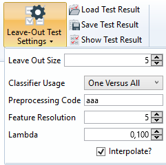
Test Results for String Labels (Classification)
After performing a test (Sample Test or Leave Out Test ) the results will be shown immediately. They may also be displayed once a test has been performed (or an existing results file has been loaded) by clicking Show Test Results tool at the far right end of the Polimago CR ribbon menu.
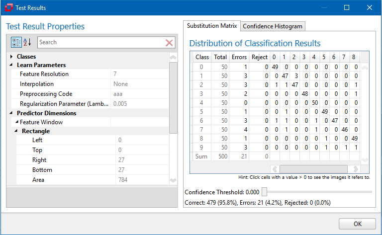
A click on any enabled field of the confidence matrix brings up a detailed list of the samples belonging to the cell that has been clicked. For example a click on the "3" in the column "Errors" of line "1" reveals the three misclassifications that happened:
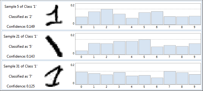
The information on the left can help locate the misclassified sample in the sample image list. Next to that a sample is shown and to the right a histogram shows the confidence distribution among the different available classes (in this case for all three samples the classification result was not clearly cut out - the (wrong) result just happened to be slightly better than all the others).
Note that the class information always refers to the sample image list the test result has been created from. Once the sample image list is altered, the information looses validity and the displayed images may in fact become misleading!
The Confidence Histogram in the second tab visualizes the amount of correct classified items (shown as green bars) compared to the classification errors (shown as red bars) depending on the result's confidence value.
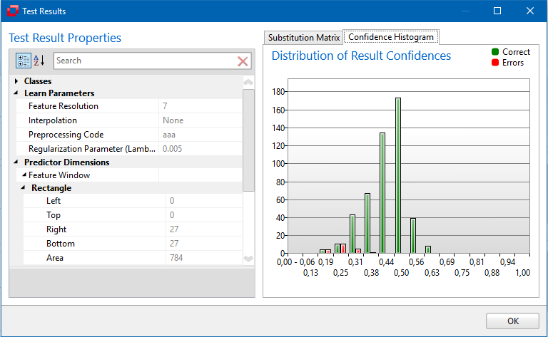
Test Results for Vector Labels (Regression)
When working with vector labels, the test results are different. Instead of the substitution matrix, a scatter plot will be shown. In this plot, the horizontal axis indicates the result's true label for the selected dimension, whereas the vertical axis shows the regression result(s).
Therefore the horizontal axis will in practice never be densely populated, and the data along the vertical axis will always be spread out to some extent. Rather than display all the individual results (which would result in a fairly unreadable graph), the TeachBench visualizes the distribution of results by showing indicators for the median and the 50% and 90% quantils. The ideal graph would of course show a very narrow distribution that closely aligns with the diagonal line.
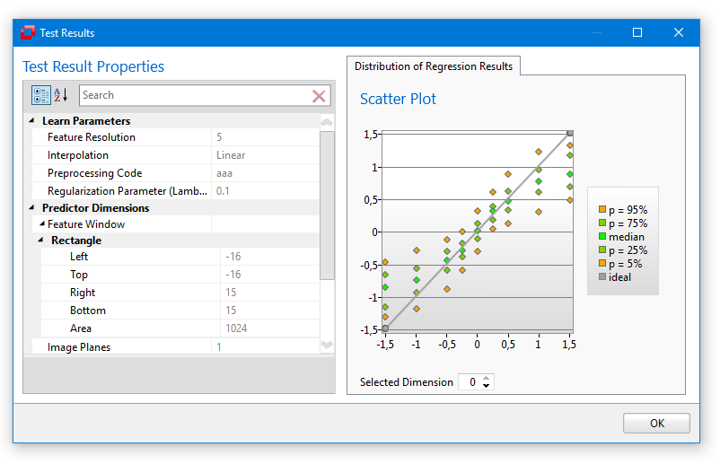
As long as there are no inconsistencies in the sample image list, introduced either by mistake or due to extremely poor image quality, there can never be too many samples in a sample image list (in theory that is). But, memory restrictions apply - keep in mind that in a 32 bit process the available address range amounts to 2 GB, 3 GB tops and that the training data shares the available address range with other DLLs. Additionally, the process needs adjacent (contiguous) memory for many of its tasks. In practice about 500 to 600 MB seems to be the upper limit for a sample image list in a 32 bit application. If more memory is required, it is recommended to use the 64 bit build of Polimago CR. It is also important to point out that the processing time a classifier needs at runtime does not depend on the number of sample images (in other words: more training on a classifier will never hurt). If a classifier generated from 10 images takes 40 ms to search an image, a classifier generated from 10000 images with the same learning parameters will take 40 ms to classify a sample as well. And down to a problem-dependent saturation point, adding more samples can only improve the classifier. In most applications we found a polynomial dependency of the error rate ε on the inverse of the sample number n, very often ε being proportional to roughly 1/√n, a fact related to the law of large numbers in statistics. This dependency persists up to some saturation point, where the decrease of ε slows down considerably or e becomes constant.
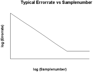
Nevertheless, the error rate at the saturation point is often very low. A case in point is given by our studies of the MNIST database, a standard benchmarking set for pattern recognition systems in which the patterns are hand-written digits from 0 to 9 collected by the US-national institute of standards. There are 60000 training samples (6000 per class) and 10000 test samples:
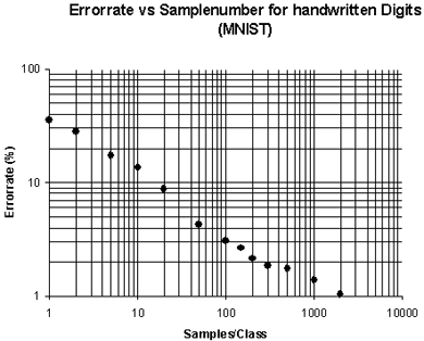
Despite the enormous number of training samples, we didn't get to a saturation point, even though there is a decrease in improvement and a significant departure from the 1/√n-behaviour as the error rate sinks below 2%. For the full training set with 6000 samples/class Polimago CR arrives at error rates around 0.8%, which compares favorably to the best results obtained with other techniques (within the accuracy limits imposed by a modest testing set of only 10000 samples). The bottom line is: In a well defined problem don't worry about saturation, but prepare as many training samples as possible.
Confirmations
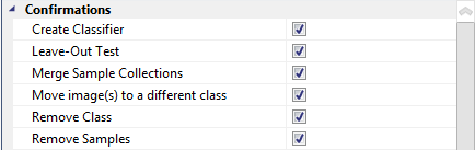
Here you can toggle the confirmation notifications. They will (or will not if you chose so) be shown if you remove a class or one or several samples or if you create a classifier or start a leave out test since these two operations might take a considerable amount of time. There are also confirmations available for merging sample collections, moving images from one class to another or removing entire classes or (one or several) samples.
Learning Parameters
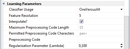
Here all parameters relevant for classifier creation are shown. Besides the read only parameters that are merely shown as an information for the user, the parameters are the same that can be accessed via the Learning Parameters menu or the Leave Out Test Parameters menu from the Polimago CR ribbon. For details see Multi-Resolution Filter and Lambda, Feature Resolution and Interpolate.
Testing

Here you can set the bag size of the Leave Out Test (see Testing a Classifier).
One of the most common tasks in machine vision is the recognition and location of objects in images. This process, commonly referred to as pattern recognition, is used in a wide range of applications either to locate a product in the image before applying further tasks such as gauging or identifying defects or by classifying an object into a number of known variants.
The main focus of Polimago Search is therefore the robust search for trained objects in images. With its sophisticated algorithms, the tool is not only capable of finding the position of a trained object, but also of retrieving the orientation and the scale of the object. On this note, this tool is predestined for the robust recognition of object poses and the tracking of different objects in image sequences.
Other benefits of this tool are the easy teaching process which does not need much user input and its outstanding performance which makes the tool a good choice for real time applications.
This section is divided into several sub-sections which cover the main aspects of Polimago Search:
To achieve robust recognition results pattern recognition largely depends on the tolerance to variability of the teaching model. Variability is therefore an indicator of how good the detection rate of a pattern is under varying conditions such as illumination levels, object scale, orientation, tilting, shadows and partial occlusions.
Fixed single pattern approaches while fast and easy to teach often only cover a small range of variations and therefore achieve low recognition results under varying conditions. Polimago Search establishes a new training strategy which is based on a variable teaching model and does not need any additional user input. The following sub sections will explain the different aspects of this new technology.
Terminology
The following terms and definitions are specific to the Polimago Search module. For an additional list of definitions applicable to all the available TeachBench module please refer to the Definitions section.
Model
A model serves as an entity which describes a pattern to be learned by the algorithm. A model is formed by one or more images from the pattern. Please see the section Creating Models and Instances for details.
Search / Search Classifier
A Search function which finds the pose of the trained pattern in the image. The initial search is carried out within a coarse grid called Grid Search. Each position is inspected by the Search Classifier. For more information please see Description of the search stage further down in this section. The Search classifier is the result of Polimago's learning stage.
Pose
The pose is the result of a successful search and describes the geometric alignment of the pattern relative to the position of the camera. The pose normally consists of a two-dimensional position x,y, expressed in pixel coordinates, an orientation in radians and a scale where 1.0 means no scaling (original size). Extended modes of Polimago Search can also deal with affine pose parameters of the pattern. For more information please see invariance type.
Invariance Type
The amount of information a pose consists of is defined by the invariance type. This parameter has to be set in the learning stage of a Polimago Search classifier. A detailed description of all parameters of Polimago Search can be found in the section Creating a Classifier.
Description of the learning stage
The operating principle of Polimago Search is based on the two-step-operation common to every tool in pattern recognition:
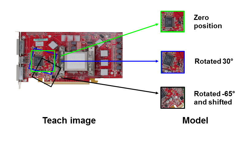
Given a single pattern image or a collection of pattern images, the user creates a teaching model by placing a feature window in the image - this window is indicated by the green rectangle in the figure above. This is the only user interaction needed since all the following steps are now performed automatically by Polimago's learning algorithm.
Description of the search stage
The goal of the search stage is to locate the trained model in the given image and to retrieve further information about its pose. To achieve this, Polimago Search superimposes a grid structure on the image which is illustrated in the following figure (green rectangles rectangles represent the feature window drawn around each of the grid points). For every grid position a regression based metric predicts if there is a match in the region or not. If a match exists, the search is traced to the final pose of the found object.
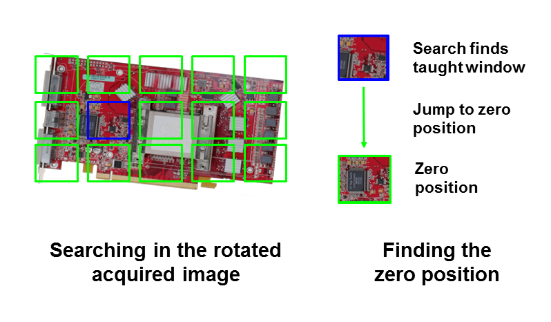
According to the example the grid search succeeds in one of the feature windows (which is marked with a blue rectangle). Since the algorithm of Polimago Search has learned this window during the learning stage the search classifier can jump immediately to the zero position of the pattern and retrieve its pose information. A key advantage of this strategy is the ability to speed up the search process by only searching in a fairly coarse grid in the image. This makes Polimago Search suitable for real time applications, for example tracking tasks.
This section describes the main steps involved in building a Polimago Search project including pattern image selection, model and instance creation and classifier training and testing. Each of the following steps is described in detail with text and images:
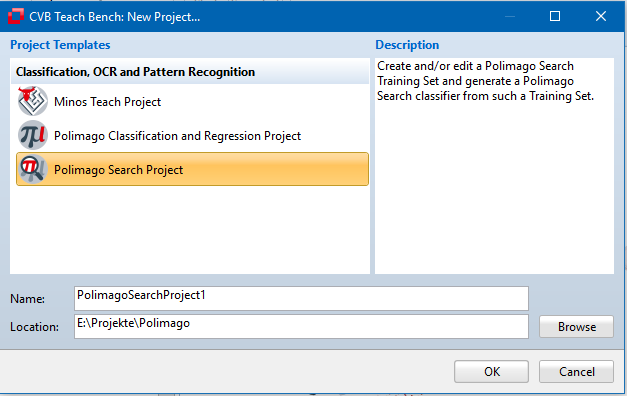
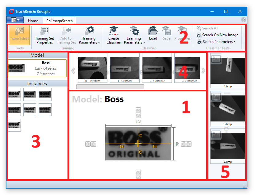
As always, the TeachBench's application main holds the functions to Save the current project or to Load existing projects from your hard disk. Polimago Search project files use the extension .pts (short for Polimago Search Training Set).
Since we are dealing with a tool for pattern recognition we need images. The basis for the teaching process is therefore the image pool which serves as a hub for all images available for training and/or testing. Images can be added to the image pool via the main menu - Open - Image or Video:
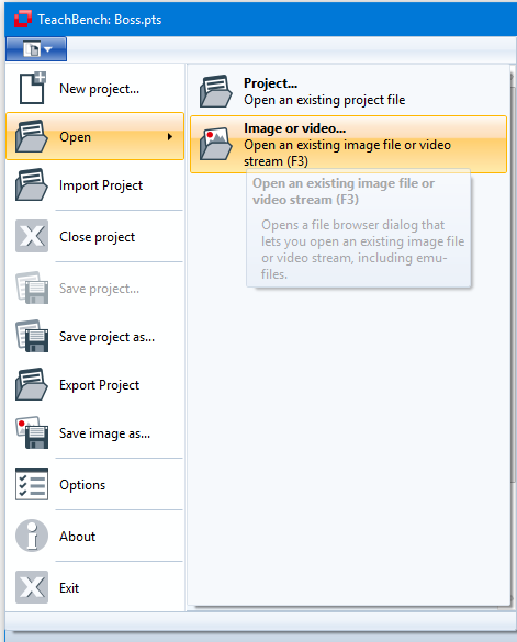
The dialog allows you to open a variety of different image and video formats. After selection, the images are visible in the Image Pool which is located on the right hand side of the workspace:
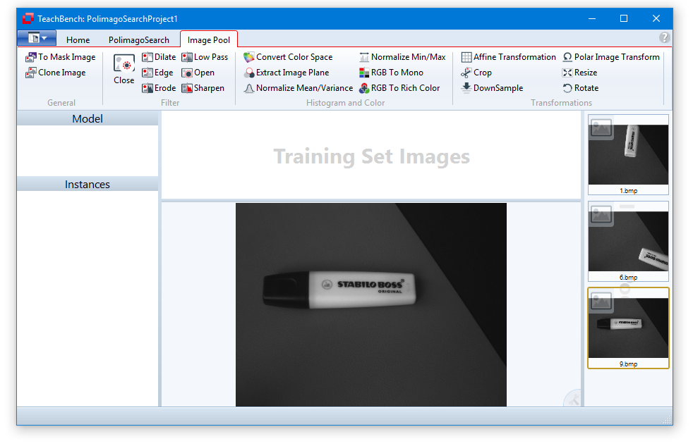
In the example we added three pattern images to the Image Pool. In general, it is good practice to add several images of the pattern to be recognized to the training of a Polimago Search classifier. This can make the classification more robust since variations in the lighting condition, shadows etc. can be better compensated if the training is based on more than just one scene. To achieve good classification results it is recommendable for the different pattern images to have the same orientation and scale.
In order to start the training, the images need to be added to the Training Set (button at the Polimago Search ribbon tab). Please note that the Polimago Search module only expects gray value images for the training (as of now) - in case the images in the pool are color images there is a function which provides the conversion to gray value images:
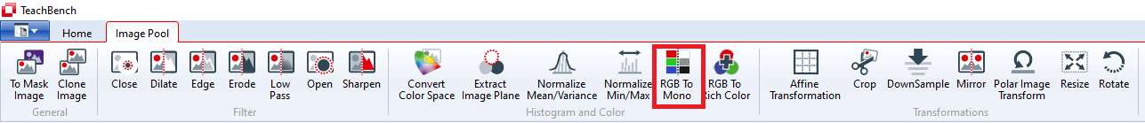
Moreover, the Image Pool's ribbon tab provides a number of different image processing tools like:
The operators that have already been applied to an image can be shown in the processor stack view, where it is also possible to modify the order in which they are applied and their parameters:
Now it is time to create a model. Generally, a model tells the search classifier of Polimago what to search for in the images. This is specified the feature window. Since we are interested in the lettering "BOSS original" of the image we click in the middle of the lettering:
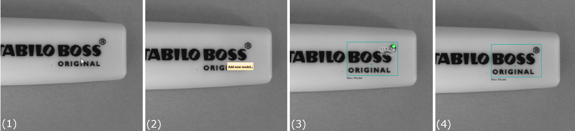
Through those four steps a new model with one instance has been created and is now visible in the left corner of the Training Set Images Region. Clicking on the model allows you to see and edit the model's feature window (extent and reference point) using the arrow buttons on either side or dragging the reference point crosshair:
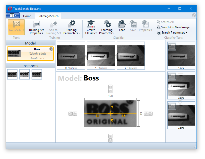
Unlike the Minos or Polimago Classification and Regression module Polimago Search allows you to define only one model at a time. The reason for this lies in the search algorithm which is only capable of searching for one specific model in an image. If a differentiation between different object types is one of the goals in the application, a Polimago Classification and Regression classifier will be needed for an application-specific follow-up step.
A model of the Polimago Search algorithm can deal with different variations of a pattern. To achieve this invariance, a model should normally be built of more than one instance. In our example we added two more instances of the "BOSS" lettering to achieve better search results during varying lighting conditions. This was done by adding the next two images of the pen to the training set by clicking on the "BOSS" lettering and selecting the previously trained model.
Please note that the image that is shown as a thumbnail for the model shows an average image over all instances or just the first instance (this may vary depending on the current state of the application). This image does not represent the "model" that is used for the algorithm, it's just for visualizing purpose.
Creating a search classifier that returns accurate data about an object's location and pose requires accurately positioned training instances. To aid the user in generating these, the Polimago Search module offers the same feature found in the Minos Module: When a location in the image is clicked to define a new instance for the Polimago Search model, a correlation between the average of the instances trained so far and the surroundings of the newly clicked instances can be calculated to find the optimum position of the new instance. This correlation step can be configured using the parameters accessible via the ribbon button Training Parameters:
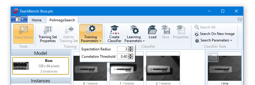
The currently trained instances can displayed by selecting (clicking) the Polimago Search model. In the example below, that three instances of the model are available now:
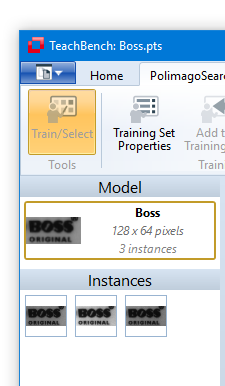
Once the model and instance creation is complete we may proceed to the creation of a classifier in the next section.
Training Set Properties
Once a training set has been created, you can review the training set properties via the corresponding button from the ribbon menu (left most at the Training section). Clicking this button will open a dialog window that shows various information regarding the currently loaded training set.
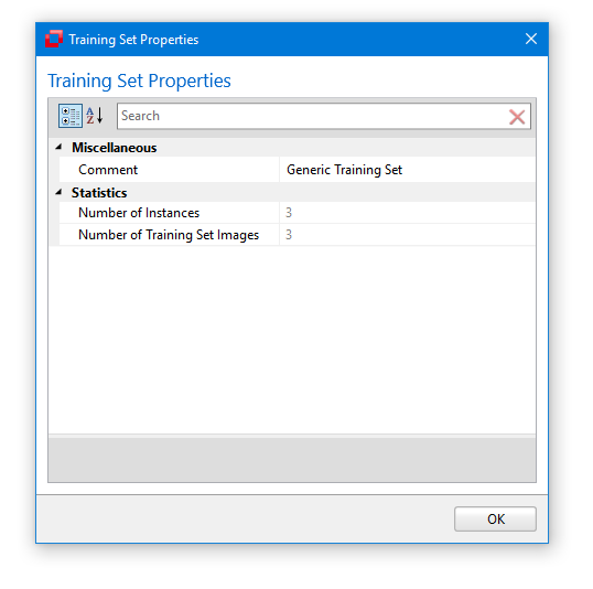
After defining the model and adding enough images (and instances) to the Training Set we may proceed with the creation of a Polimago Search classifier. Depending on the learning parameters, learning a Polimago Search classifier can be a fairly time-consuming process. So, it makes sense to familiarize yourself with the available parameters before delving into classifier creation. The learning parameters are accessible through the accordingly named ribbon button , but also through the Polimago Search module's options window.
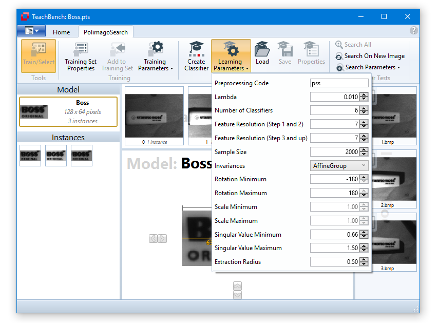
The preprocessing code is a string which can consist of 4 different characters. With the exception of '+' they correspond to processing operations and are executed from left to right (see also the description of the Multi-Resolution Filter in the Polimago Classification and Regression module).
Lambda (Regularization Parameter)
The parameter Lambda specifies the ridge regression regularization value. The default value 0.1 works well in most cases. It should be slightly increased for a small number of training examples and slightly decreased for a large number of training examples.
This parameter controls the number of steps carried out in the elementary search process. The default value is 6.
The parameter Feature Resolution 1-2 controls the resolution for the first two estimates in the search process. Smaller values lead to a coarser resolution. Normal values range from 3 to 8. For a description of the effect of the Feature Resolution settings please refer to Lambda, Feature Resolution and Interpolation in the description of the Polimago Classification and Regression module.
The parameter Feature Resolution 3+ controls the resolution for the third (and all following) estimates in the search process. Smaller values lead to a coarser resolution. Normal values range from 3 to 8. For a description of the effect of the Feature Resolution settings please refer to Lambda, Feature Resolution and Interpolation in the description of the Polimago Classification and Regression module.
The parameter Sample Size sets, the number of learning examples to be considered (the number of instances that have actually been marked will be boosted up to the given Sample Size by randomly transforming the trained instances within the invariance limits given further down). The default value 2000 is a good compromise between learning time and accuracy. For difficult problems with 4 or 6 dimensional invariance a larger value may be required. This considerably increases the learning time (3rd power of sample size), but does not affect the execution time of a search.
The amount of information a pose consists of is defined by the Invariances. Different modes are:
Gives the minimum and maximum scale at which learning samples will be generated (and therefore also roughly the minimum and maximum scale that the classifier will be able to identify). The value Min Size specifies the scale-invariance of the classifier by adjusting the minimum scale of the pattern to be trained. Although a wider range of value is accessible, it is not recommendable to exceed the range [0.5 ... 2.0].
Defines the range of rotations to be learned. Angles are given in degrees and must not exceed the range [-180° ... 180°].
When generating learning samples with the invariance Affine selected, Polimago will generate random 2x2 matrices to transform the originally trained instances with. To prevent singularities, these matrices are restricted through the scale and rotation ranges already explained, but also by restricting the limits within the singular values of the matrices may lie. The further away from 1.0 the singular values of a matrix lie, the more extreme the transformation will be.
When generating samples for the learning process, the Polimago algorithm will shift the specified feature window in the image in x and y direction within the limits defined by the Extraction radius. The Extraction Radius is given in terms of the minimum of the feature window's width and height and by default is set to 0.5. Higher values for the Extraction radius will later on allow for a higher grid spacing during search operations (see Testing a Classifier) which in turn will result in a faster overall search. However, the Extraction Radius should generally not be set larger than the "typical" surroundings of an object.
An example: if the feature window is defined as 20x20 pixels with the pattern position at the center, learning examples are generated by shifting the window randomly by no more than 10 pixels in each direction. One can also express it like this: The value of 0.5 means that the algorithm can estimate the object's state if it sees only half of it. A value of 0.25 would mean that the algorithm needs to see 75% of it.
Hitting the button Create Classifier starts the training and a progress indicator with an estimate of the remaining time appears in the middle of the workspace. If the training fails, an error will be displayed in the application's status bar. Via the buttons Save and Load it is possible to save the current classifier or to load an existing classifier form your hard disk. After successful training, the classifier's parameters can be accessed via Properties (button ):
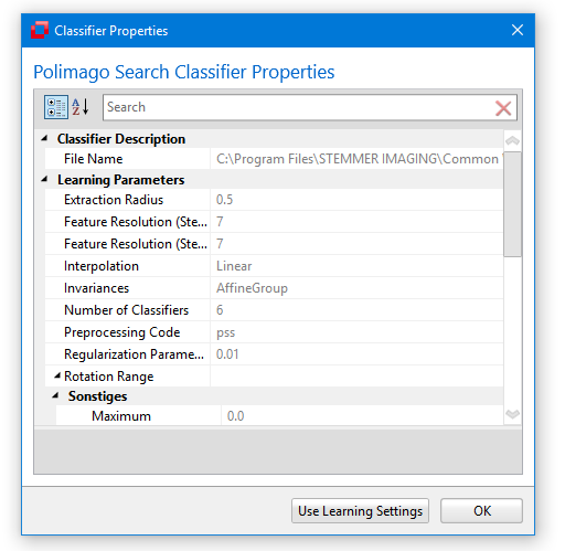
In order to test a classifier the TeachBench offers functionality to search for the trained pattern in a given image. To use it, add a new image to the Image Pool. In our example we are using the classifier trained and learned in the previous sections on a new image of a text marker which has been slightly rotated and scaled:
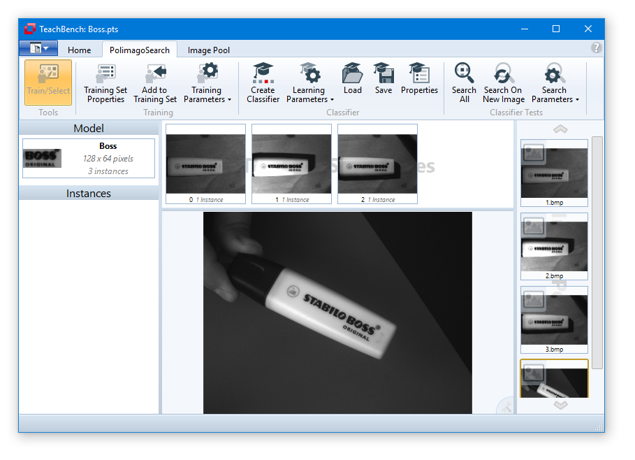
Before carrying out a search by using the Search All tool , let's review the available search parameters (accessible through the Search Parameters button in the ribbon as well as through the Polimago Search module's options dialog):
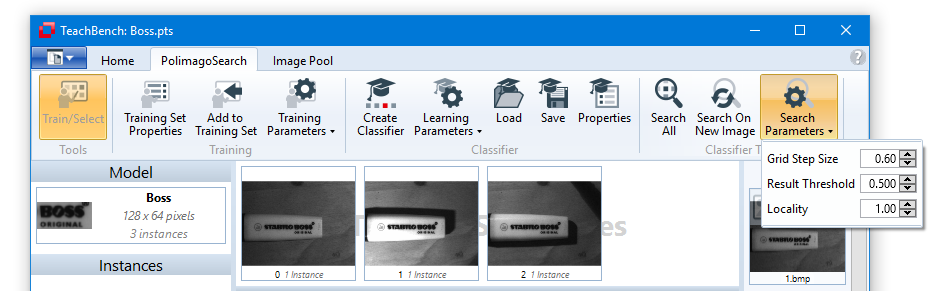
Grid Step Size
The parameter Grid Step Size specifies the step size of the grid that the function PMGridSearch() superimposes on the image. Grid Step Size is (like the Extraction Radius) given in units of the size of the feature window (more precisely the unit is the minimum of height and width of the feature window) and defines the spacing of the grid points that are going to be evaluated (needless to say that the grid size has a huge impact on the perceives speed of the classifier). Note that it is usually a good idea to have an overlap between the Extraction Radius and the Grid Size by e.g. setting the former one to 0.6 and the latter one to 0.5 (if no such overlap is given, gaps between the classifier's "knowledge" and the search grid will occur that are likely to give rise to false negatives, i. e. objects that are missed during a search operation).
Result Threshold
The Result Threshold specifies a minimum quality for acceptable solutions. The default value 0.5 is a good starting point. Note, however, that for difficult applications reasonably good results may sometimes have quality values below 0.5 (but above 0.0).
Locality
The Locality controls how closely together valid solutions may be located to each other. This parameter is, again, given in terms of the classifier's feature window (i.e. a value of 0.5 for example means that no two results may overlap by more than 50%).
After setting the Search Parameters, the search can be initiated by hitting the button Search All :
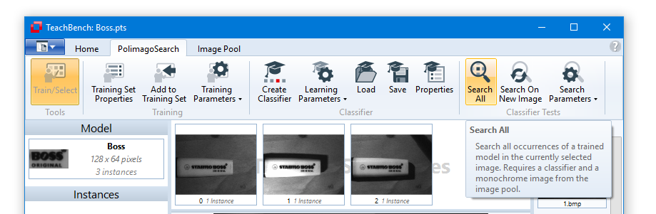
As expected the new image in the pool is searched and the result is displayed as a green frame (color can be changed in the TeachBench options) that gives an estimate of the feature window projected to the result:
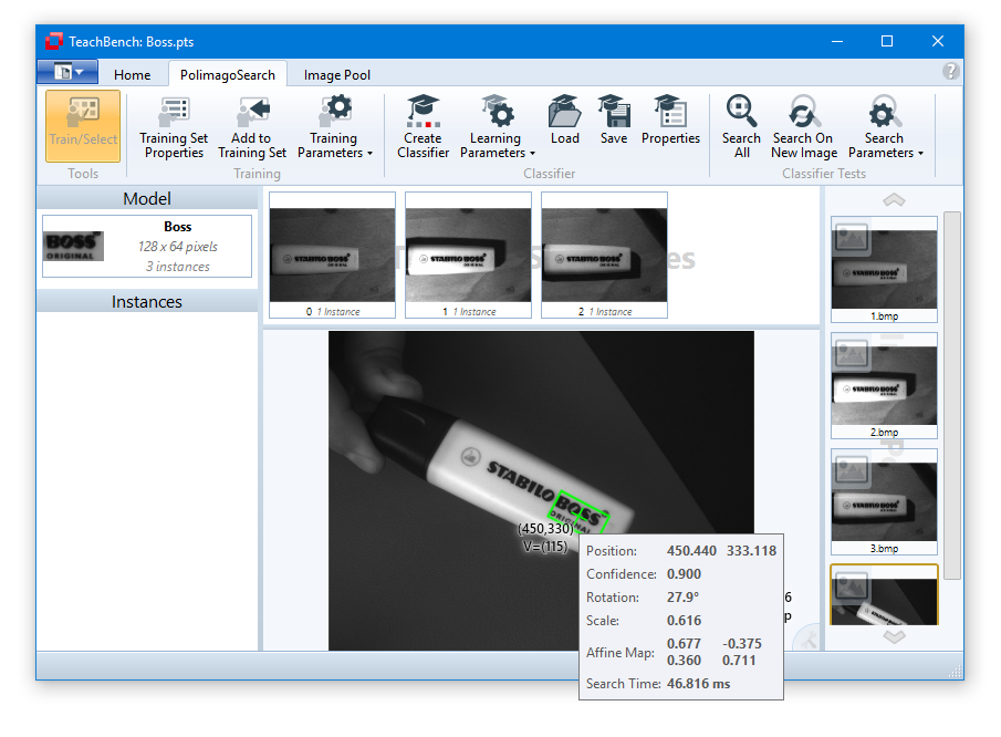
Hovering the mouse above a green frame opens a tooltip with detailed information about the current search result (position, confidence, transformation parameters and search time.)
All options for the Polimago Search Module described previously may also be accessed trough the TeachBench's main menu item Options:
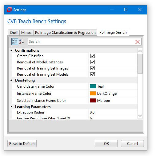
The available settings are divided into the following groups:
In this dialog, it is also possible to reset all the parameters that refer to the Polimago Search modules to their default values, using the button Reset to Default.
Further information about the use of Polimago Search for your specific project can be found in the Polimago documentation located in your Common Vision Blox installation under CVBDoc/Polimago.chm.
In this document you will find more detailed information about:
Common Vision Blox DNC is a CAD-based 3D-object recognition tool. It allows to locate objects, which are described by a CAD file, in point clouds. Only the geometric properties of the object are taken into account, its color and texture do not matter. This is where the name of the tool comes from: Depth No Color.
DNC is a two-stage detection tool. In a first step, the CAD object to be found is trained. This teaches how the object will later be visible to the sensor. After learning is complete, the second step is to detect the object in point clouds.
For the purpose of detecting objects CVB DNC tests several templates for their appearance within the depth image of a 3D-sensor, using a similarity measure composed from oriented 2D- and 3D-features. These features are calculated both for the templates and the sensor's depth image. Whenever the similarity measure exceeds a certain threshold, a hypothesis is generated, indicating a possible hit at this location within the depth image. The hypotheses are verified by optimizing the 3D-pose at this location and calculating a final similarity score.
The templates, also denoted "samples", are generated from a CAD model, which contains the object's geometric mesh data. To achieve this, an artificial sensor is pointed at the object and an artificial view of the object is calculated from its mesh data. Different views can be accomplished by either rotating the object in front of the sensor, or changing the sensor position, or both. The range of different views must cover the range of possible poses of the object which appear later on during detection. Obviously this can only be done in a discrete way, resulting in a finite number of templates.
In the following images you can see the objects mesh data, the position and looking direction of the artificial sensor and the generated sample, which serves as one template during the detection state.
|
The CAD object and the positioning of the artificial sensor. |
The sample generated from the current sensor settings serves as one template. |
During a detection task the template produces a strong detection signal wherever an object in a similar pose exists within the sensor's depth image. This region is subject to further investigation to decide if it is a true hit.
|
Original point cloud |
|
DNC-adapted depth-image with constant, distance-independent lateral resolution |
|
Spatial distribution of the hypotheses score for a matching template |
|
Spatial distribution of the hypotheses score for a matching template |
This way we create as many templates as needed to cover the range of expected poses. One single generated template covers a certain range of poses that differ by a few degrees of rotation around all axes. To detect a larger range of poses, it is usually quite sufficient to generate samples in 10 degree increments. If we have no information of the expected objects poses, we must cover the complete pose sphere around the object, including camera roll, resulting in possibly thousands of templates. But usually the space of expected object poses is constrained and the number of needed samples is limited to a few hundred. See Creating a New Project and Creating Samples for an explanation how to load a model and how to create artificial sensor views.
In order to detect objects in a point cloud, a so-called classifier is generated from the entire set of samples. In this teach process the samples are analyzed and their characteristic features are calculated. The classifier is then applied to a point cloud. For the objects found, the position and orientation are determined as accurately as possible. A geometric hash value is used as a confidence value. For all hits above the confidence value, additional values for completeness, possible occlusion and model inconsistency are determined using a precision threshold. Based on these values, a final selection of hits can be made. See Creating a Classifier and Testing a Classifier for an explanation how to use the generated samples for object searching.
This section describes the main steps involved in building a DNC Find project including sample generation from a CAD model and classifier training and testing.Each of the following steps is described in detail with text and images:
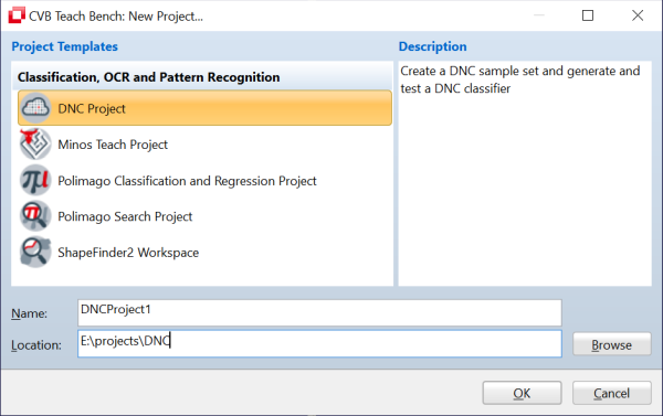
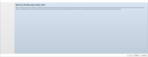
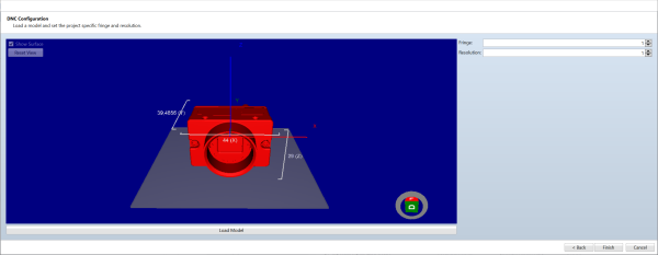
As always, the TeachBench's application main window holds the functions to Save the current project or to Load existing projects from your hard disk. DNC project files use the extension .dsl (DNC sample list).
Considerations for the choice of Resolution- and Fringe-parameters
During project creation you are prompted to choose values for the parameters Fringe and Resolution. They both influence the effectiveness of the generated samples.
Resolution
The generation of samples, which serve as templates during the search process, is done with a specified and constant spatial resolution. It is given in pixels per Millimeter and specifies the point density that the generated templates exhibit. In the training process this resolution is transferred to the classifier, which accordingly adapts the actual sensor resolution during a search process. For this reason the teaching process in DNC is independent of the 3D-sensor which is actually used later on. Some considerations should be made in order to choose a reasonable value of this resolution value:
You can visually check the quality of the generated templates. Relevant details should be visible while template size stays reasonably small.
|
A very poor resolution of 0.5 pix/mm. Details are too coarse, template size is very small (24x25) |
Optimal resolution of 2.0 pix/mm. Details are clearly visible and template size is still small (92x96) |
Very high resolution of 5.0 pix/mm. No apparent advantage in detail resolution, but a very big template size (230x240), that will probably reduce performance. |
Fringe
In most cases it is advantageous to add a fringe to the templates to ensure a proper extraction of the object's silhouette. This contributes to a reliable localization of the object boundaries during a search process. The fringe is given in Millimeter units and effectively adds a border around the generated templates of the size of Fringe*Resolution pixels. Generally a fringe size of 5 to 10 pixels is advantageous for proper object detection.
After creating a new project we are ready to generate samples. For sample generation you need to specify a sensor position and the orientation of the object in front of the sensor. The chosen situations during sample generation should resemble the real situations as close as possible. To start with sample generation, click on Generate Samples..., which opens the sample generation dialog.
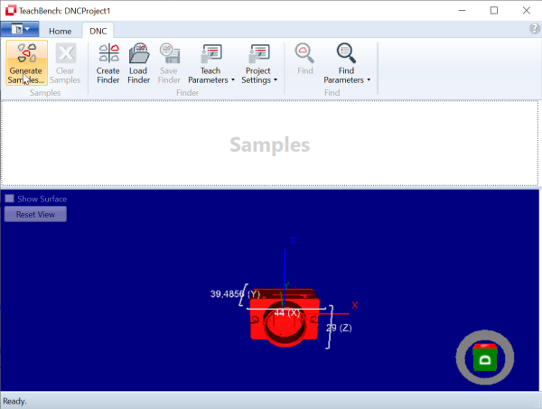
In the sample generation dialog you can specify the object's orientation and the sensor position by entering corresponding values in the left pane for Model Rotation and for Simulated Camera Position. In the view port on the right you can observe the resulting scene.
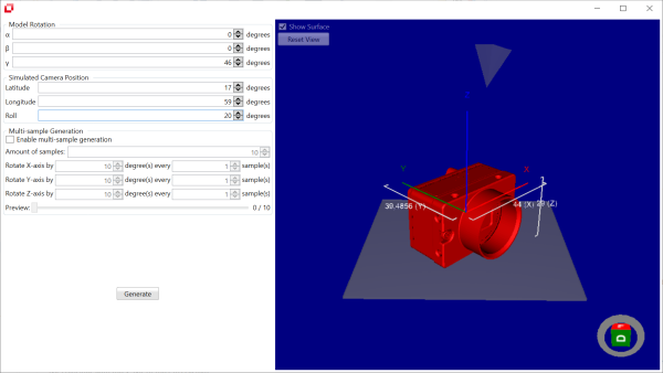
Model Rotation
You can manually rotate the model around the coordinate axes by specifying a corresponding Euler angle value for each axis. Please note that the rotation is not around the origin of the CAD coordinate system, but around a coordinate system that has the same orientation as the CAD system but has been moved to the geometric center of the object.
Simulated Camera position
The camera position is defined as a point on a sphere around the geometric center of the object. The viewing direction of the camera is always directed to the center of the sphere, the sensor orientation is upwards, i.e. for any position outside the two poles the vertical sensor axis points towards the north pole. North and South pole are two corresponding points on the Z axis of the CAD system. When the sensor is placed in one of the two pole positions, it is oriented so that the horizontal sensor axis coincides with the X axis of the CAD system. The precise position and orientation of the sensor is determined by specifying a latitude, longitude and roll angle. The roll angle represents a rotation of the sensor around its viewing direction to the center. The latitude starts at 0 degrees in the North pole and goes along the specified longitude to the South Pole at 180 degrees. The prime meridian (zero longitude) is defined as the meridian passing through the positive X axis of the CAD system.
By clicking on the Generate button, a sample for the current displayed situation will be created. When you close the sample generation dialog the created sample will appear in the Samples-area of the project.
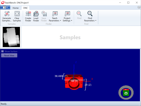
You can select the newly generated sample by clicking on it (deselect by holding Ctrl pressed during click). For the selected element the information is displayed with which parameters it was created. Furthermore, the point cloud corresponding to this sample is displayed in a new viewport. It is possible to switch between a 3D view and views of the individual X,Y,Z planes. In the Planes view, the size of the generated template can be determined by moving the cursor into one of the images. This is a good opportunity to check if the selected values for Resolution and Fringe are suitable for the project. See Fringe and Resolution for considerations regarding these values.
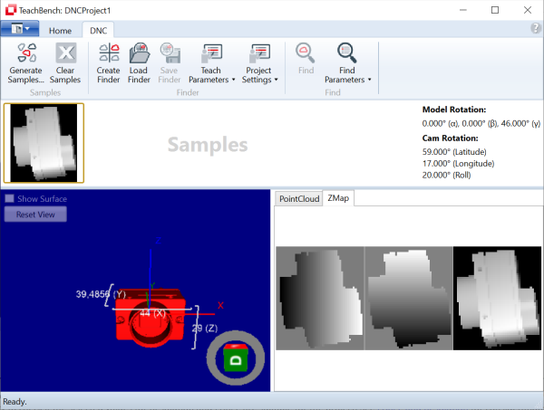
Multi-sample generation
To simplify the generation of many samples, there is a possibility to automatically generate a defined number of samples while incrementally changing the Euler angles. In the Sample generation dialog, check the Enable multi-sample generation check box, enter the number of samples to be generated, and specify how the Euler angles should change after each generated sample. For example, if you select 36 as the number of samples to generate and specify the following settings, a full 360 degree rotation around the Z axis will be simulated in 10 degree increments. By moving the Preview slider, you can study the motion sequence that the object will go through.
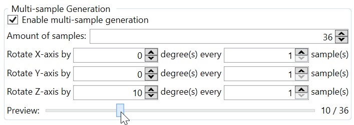
In the Samples-area, you can delete a selected sample by clicking on its delete-button. The Clear Samples button will remove all samples from the Samples-area.
Clicking Create Finder creates a classifier from the entire set of samples.
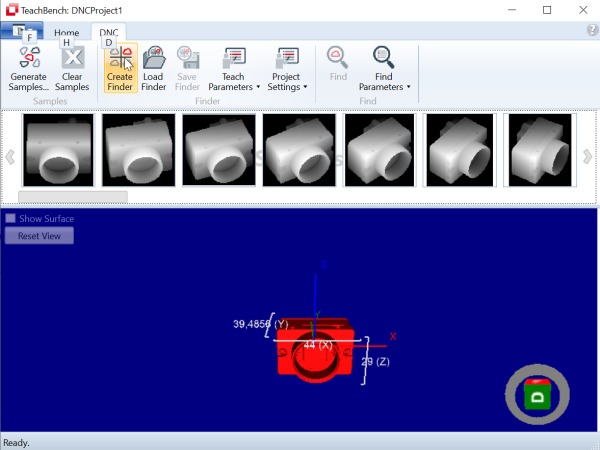
This process extracts the characteristic features of the samples and arranges them in a way that allows quick calculation of similarities in point clouds. The choice of the Teach Parameters influences these calculations, which in turn have a great impact on the effectiveness of the classifier.
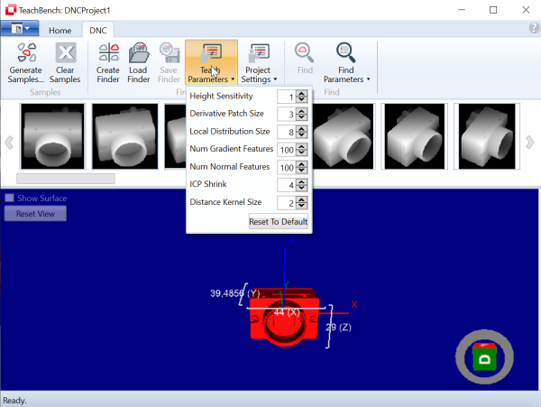
See Teach Parameters for an explanation of this parameters. The resulting classifier can be stored into a separate file with Save Finder and reloaded later.
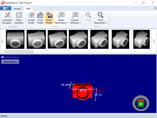
Height Sensitivity
Minimum gradient magnitude to accept a local gradient as a feature in the depth images. The value specifies a threshold (in millimeters) above which local height changes are observed as characteristic features. A typical value is 1 mm, the minimum value is 0. This value is also used implicitly during later search tasks.
Derivative Patch Size
Smoothing area in pixels for gradient and normal calculation. The value controls the local environment in the depth images of the examples which is used to calculate gradients and normals. Minimum is 3. Larger values effectively result in a smoothing of the depth images. The value should be odd. Typical values are in the range [3..9]. Smaller values should be favored, since the example images of the CAD object are flawless and free of noise. The corresponding value DerivativePatchSize in the Find Parameters of a detection task should be equal, or - in case of sensor noise - bigger.
Local Distribution Size
Size of area in which local features are distributed (in pixels). To account for the finite and discrete example positions the local features are somewhat smeared out. This value specifies the local active range of a single feature. A typical value is 8, the minimum value is 0.
Num Gradient Features
Number of gradient features retained in the classifier. To speed up the calculation of correspondences during a detection task, the possibly dense gradient features from the examples are thinned out to a minimum necessary number. This number strongly depends on the object itself. Typical values are between 100 and 1000. A value of 0 means that all gradient features should be used.
Num Normal Features
Number of normal vector features retained in the classifier. To speed up the calculation of correspondences during a detection task, the dense normal features from the examples are thinned out to a minimum necessary number. This number strongly depends on the object itself. Typical values are between 100 and 1000. A value of 0 means that all normal features should be used.
ICP Shrink
ICP-subsample factor. To speed up search tasks, a voxel representation of the examples is pre-calculated. The subsample factor determines the amount of data used to perform an ICP-operation. It strongly influences the recognition speed and the amount of memory used. The recommended value is 4. The minimum value is 1, resulting in no subsampling.
Distance Kernel Size
Factor for Distance transform calculation. A so called Huber kernel is used for the calculation of a distance transform of an example. To some extend a Huber kernel bigger than 1.0 can possibly enlarge the convergence basin of ICP-operations, relative to the Euclidian distance transform (Huber kernel = 1). The recommended value is 2.0, the minimum allowed value is 1.0.
This feature allows you to test a freshly created or reloaded classifier on a given point cloud. To use it, you must first load a point cloud and display it in the viewport. All loaded point clouds are listed in the right column in the Pointcloud-Pool area.
 To load a point cloud, click on Open/Load image... To load a point cloud, click on Open/Load image... |  All loaded point clouds will appear in the Pointcloud Pool. All loaded point clouds will appear in the Pointcloud Pool. |
When you load a point cloud file (tif), you are asked whether the file should be interpreted as an image or as a point cloud. Select "No" in the corresponding "Duplicate file type" dialog.
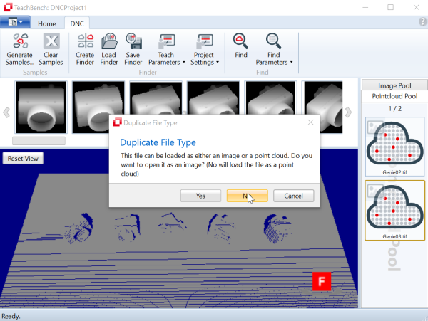
See Point Clouds and Frame Orientations for more information on the supported file types.
When the point cloud is visible in the viewport click on Find. DNC will perform a search operation and mark the found objects in the point cloud. Each object found is drawn in its position and orientation as an overlay in the point cloud. In addition, the CAD system is drawn in its corresponding position.
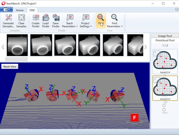
To display the information of a found object, it can be selected by clicking on it. The position, orientation and score of the individual object are then displayed in the lower left corner.
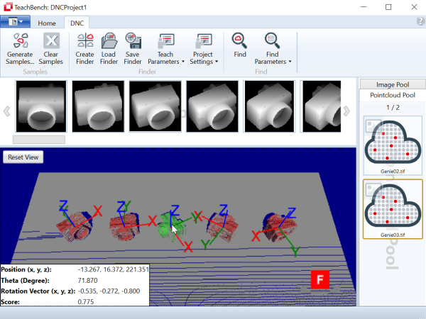
If the objects are not found as expected, it is recommended to adjust the Find Parameters accordingly. As a first step, Raw Results Only should be checked and the search operation repeated. This has the effect that all candidate regions that exceed the Hypotheses Threshold are displayed. You can experiment with the Hypotheses Threshold until all objects and as few false positives as possible are found. Then reset the Raw Results Only switch. If objects are still not found, increase the values for Precision Threshold, Max Occlusion and Max Inconsistency and decrease Min Coverage and Min Score, until you achieve a satisfactory result.
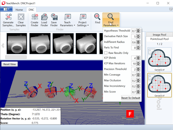
Hypotheses Threshold
Minimum feature score for hypotheses generation. The value controls which areas of the depth image are used as candidates for closer examination. The feature score is calculated from the correspondences of gradients and normals between all models and the actual point cloud data. The threshold should be chosen so that on the one hand all object candidates are found, on the other hand as few false candidates as possible are generated. Typical values are in the range between 0.9 ... 1.0. Disturbances in the point cloud, missing or spurious data may make it necessary to reduce the value. The minimum value is 0.5. To find a usable threshold it is recommended to set the flag Raw Results Only.
Derivative Patch Size
Smoothing area in pixels for gradient and normal calculation. The value controls which local environment in the depth image is used to calculate gradients and normals. Minimum is 3. Larger values result in a smoothing of the depth image. The value should be odd. Typical values are in the range 3..9.
Indifferent Radius
Fraction of template size which accounts for a single object. The value specifies within which vicinity of a found candidate no further candidates are searched for. The value 1 indicates the largest extent of the learned object. For elongated objects that are close to each other, a smaller value may have to be selected. The minimum value is 0.5.
Parts To Find
Maximum number of objects to find. The value specifies the maximum number of objects to be detected. A value of zero means that all objects should be found.
Raw Results Only
Report all regions with a score above the Hypotheses Threshold as hits. If this flag is set, candidate locations are considered hits without further investigation of these candidates. In this case, only the parameters Hypotheses Threshold and Parts To Find are decisive for finding objects. Note that the resulting values for the poses (position and orientation) are only rough in a sense, that no fine tuning (ICP) takes place. Also, in this case the reported Score values coincide with the feature scores, which makes it possible to determine a useful value for Hypotheses Threshold.
ICP Shrink
Subsample factor for ICP. The value specifies the factor by which the number of 3D-points within the area of a found candidate is reduced before the exact position of the object is determined by means of an ICP algorithm. The minimum allowed value of 1 means no reduction (highest accuracy). With increasing reduction, the processing speed increases, but at the same time the accuracy of the results also decrease. Typical values are in a range 1..4.
ICP Max Iterations
Maximum number of ICP-iterations. The value specifies the maximum number of iterations of the ICP algorithm. Increasing the value may increase the accuracy of the result, while possibly increasing the processing time. A typical value is 10.
Precision Threshold
Maximum allowed distance for local deviations (in mm). The calculation of the result score is based on deviations between the CAD model and the point cloud data. This value determines which deviation is considered tolerable, inconsistent or occlusion. The value depends on the quality of the point cloud data. A typical value is 2 mm, the minimum allowed value is 0.
Min Coverage
Minimum required fraction of point cloud view. The value is a threshold (0..1) that specifies the minimum required coverage of the model view by the point cloud data in order for the hit to be counted. A typical value may be 0.8. It is influenced by Precision Threshold.
Max Occlusion
Maximum allowed fraction of point cloud view to be occluded. The value is a threshold (0..1) that specifies the maximum allowed part of the model view which is occluded by the point cloud data in order for the hit to be counted. Occlusion is defined to be point cloud data lying between the model and the sensor. A typical value may be 0.2. It is influenced by Precision Threshold.
Max Inconsistency
Maximum allowed fraction of point cloud view to be inconsistent with model. The value is a threshold (0..1) that specifies the maximum allowed part of the model view to be inconsistent with the point cloud data in order for the hit to be counted. Inconsistency is defined to be point cloud data which is beyond the model. A typical value may be 0.2. It is influenced by Precision Threshold.
Min Score
Minimum required final score. The value is a threshold (0..1) that determines whether the candidate is counted as a hit. For this, a hash similarity score between final model view and point cloud data must exceed this limit. A typical value may be 0.8.
DNC operates on organized calibrated point clouds. That is, the point clouds are organized like the sensor depth image, but contain actual metric X,Y,Z coordinates instead of uncalibrated distance values. Since there is no standard format for storing this data format, Stemmer Imaging has developed its own format called "dense point cloud", which is stored as a TIF file on the hard disk.
The generated CAD samples and the point cloud must be oriented equally. We have stipulated two different point cloud orientations that can be used in a DNC recognition task. They differ in the way how the sensor's depth images are oriented. We call them "sensor frame orientation" and "object frame orientation".
In sensor frame orientation, the point cloud has its origin in the very center of the sensor. The Z-axis points towards the scene and the X-axis goes to the right (the horizontal direction of the sensor). Accordingly, Z-coordinates increase with increasing distance from the sensor.
|
A depth image of a 3D-sensor which delivers point clouds in sensor frame orientation. Depth values increase with increasing distances. |
3D-visualization of point cloud data. The sensor is positioned in the origin of the point cloud. |
In the object frame orientation the point cloud has its origin in a predefined distance from the sensor, while the Z-axis points in the direction of the sensor. Accordingly, Z coordinates increase with decreasing distance from the sensor. Again the X-axis points to right, thus resulting in reversed direction of Y.
|
A depth image of a 3D-sensor which delivers point clouds in object frame orientation. Depth values increase with decreasing distance to the sensor. |
3D-visualization of the point cloud. Its origin is situated at a predefined distance from the sensor. The Z-axis points towards the sensor. |
In both frame orientations DNC considers points with positive Z-coordinates only. Thus, in object frame orientation the origin of the coordinate system must be located behind the objects to be detected. Otherwise they are invisible to the classifier. DNC automatically detects which frame orientation is present.
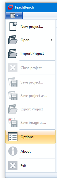
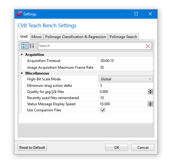
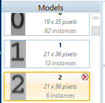
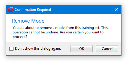
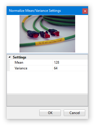
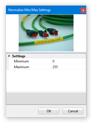
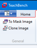
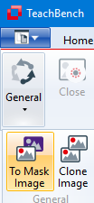


")
")
, that will probably reduce performance.")


